Download
1 / 14
140 likes | 272 Vues
U.S. IOOS Coastal Ocean Modeling Testbed. Sensitivity Analysis of Temperature and Salinity from a Suite of Numerical Ocean Models for the Chesapeake Bay. Lyon Lanerolle 1,2 , Aaron J. Bever 3 and Marjorie A. M Friedrichs 4

E N D
U.S. IOOS Coastal Ocean Modeling Testbed Sensitivity Analysis of Temperature and Salinity from a Suite of Numerical Ocean Models for the Chesapeake Bay Lyon Lanerolle1,2, Aaron J. Bever3 and Marjorie A. M Friedrichs4 1NOAA/NOS/OCS/Coast Survey Development Laboratory,1315 East-West Highway, Silver Spring, MD; 2Earth Resources Technology (ERT) Inc.,6100 Frost Place, Suite A, Laurel, MD; 3Delta Modeling Associates, Inc., San Francisco, CA ; 4Virginia Institute of Marine Science, The College of William & Mary, Gloucester Point, VA. 24 January 2011 10th Symposium on the Coastal Environment 92nd Annual American Meteorological Society Meeting
Introduction and Motivation • Physical component of Numerical Ocean models generate water elevations, currents, T and S • Water quality models and ecological models/applications rely primarily on T and S (from the physical model) • Expect “best” water quality predictions to result from the “best” T and S predictions (relative to observations) • Therefore attempt to: • examine predicted T, S sensitivity to various model parameters • optimize the predictions for T, S from models • examine how different models compare with observations and each other • employ “best” T, S predictions for water quality forecasting
US IOOS Coastal Ocean Modeling Testbed • Focus on Estuarine Dynamics and Modeling component • Ideal candidate is Chesapeake Bay: • Extensive data sets available (in time and space) • Several numerical ocean model applications available • Ocean models available for Testbed: • CBOFS (NOAA/NOS/CSDL-CO-OPS, Lyon Lanerolle et al.) • ChesROMS (U-Md/UMCES, Wen Long et al.) • UMCES ROMS (U-Md/UMCES, Ming Li, Yun Li) • CH3D (CBP, Ping Wang; USACE, Carl Cerco) • EFDC (William & Mary/VIMS, JianShen and Harry Wang) • Observed data – Chesapeake Bay Program (CBP) • Simulation period – 2004 calendar year (2005 is similar)
Model-Observation Comparison Metrics • Metric used is the Normalized Target Diagram (Jolliff et al. 2009) • m’ = m - M, o’ = o - O • σo - SD of obs. • Model skill is distance from origin (origin = perfect model-obs. fit) • Graphical versus numerical approach more informative Bias [(M-O) / σo] +1 Overestimates mean unbiased RMSD [sign(σm - σo)· {Σ (m’-o’)2 / N}1/2] / σo -1 +1 Overestimates RMSD -1
Chesapeake Bay Program Comparison Stations • Model(s)-Observation comparisons were made at 28 CBP stations • Stations covered lower, mid, upper Bay, Bay axis and tributaries
Model Calibration / Parameter Sensitivity(using CBOFS) Bottom T Bottom S Greatest sensitivity Maximum S stratification Depth of max. S strat.
Global Errors Bottom T Bottom S Upper Cook Inlet Nests Kachemak Bay • Errors were computed by considering all (28) stations at all depths and for full year • T - CBOFS best with accurate mean and error is in overestimated RMSD • – EFDC and ChesROMS underestimate RMSD and latter underestimates mean • S – EFDC, CH3D best but have opposite RMSD error; former underestimates mean • - again, errors show greater spread and larger magnitude than for T
Geographical Error Dependence (T) • Bay axis errors plotted as a function of station latitude • Errors are for bottom T • No strong dependence on geography (lower-, mid-, upper-bay) – small error spread • Different models have different skill characteristics (over/under estimation of mean and RMSD)
Geographical Error Dependence (S) • Errors are for bottom S • Unlike T, errors show greater spread • 3 ROMS models similar, have largest errors and greatest in upper Bay • CH3D, EFEC smaller errors, evenly spread and less geographical dependence
Value-Based Error Dependence (T) • Errors for bottom T plotted as the observed mean value itself • Models show similar trends with UMCES ROMS and CBOFS showing slight improvements over others • Generally, warmer T values have smaller errors – as seen by UMCES ROMS
Value-Based Error Dependence (S) • Bottom S errors show greater spread than for T • Error characteristics from models are similar except UMCES ROMS – full underestimation of mean • No consistent value-based error dependence in any of the models
Seasonal Error Dependence (T) • Errors for bottom T plotted as a function of month in 2004 • Spread in errors seen for all models – EFDC the most; warmer months have smaller errors • CBOFS is most accurate and errors well balanced • CH3D – overestimates mean, ChesROMS – underestimates mean • EFDC – largest errors during latter half of year
Seasonal Error Dependence (S) • Bottom S errors show less spread than for T • Different error characteristics in each model • 3 ROMS models show similarity – overestimation of RMSD and underestimation of mean (except CBOFS) • CH3D – underestimates RMSD • EFDC – underestimates mean and under- and over- estimates RMSD
Conclusions • Inferences for 2004, 2005 similar - so focused on 2004 • Bottom S was the most sensitive variable and was used as a proxy • Model calibration/sensitivity study showed CBOFS was not significantly sensitive to parameter variation • Global T, S errors – no drastic differences between different model predictions (although some were relatively better) • Geographical error dependence – ROMS models had largest errors in upper Bay; CH3D, EFDC less geographically dependent • Value-based error dependence – warmer T values have smaller errors; no discernible error trends for S • Seasonal error dependence – T from ROMS models are similar and CBOFS has best error balance (mean/RMSD); for S, models show different error characteristics with under/over estimation of mean/RMSD in each • Target Diagrams proved to be an invaluable and straightforward metric for studying T and S model-observation differences