Download
1 / 1
10 likes | 141 Vues
The multimodel and combined ensembles show the higher BSS and resolution (no significant differences were found for the reliability component). The pragmatic approach is better than breeding at 24 hr lead time, but is worse than breeding at 48 hr lead time.

E N D
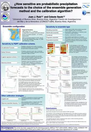
The multimodel and combined ensembles show the higher BSS and resolution (no significant differences were found for the reliability component). The pragmatic approach is better than breeding at 24 hr lead time, but is worse than breeding at 48 hr lead time. The pragmatic ensemble approach when is calibrated using the weigthed ensemble mean is equivalent to a spatial smothing of the field where the higher weights correspond to small displacements (1-2 grid points). As the maximun displacement increasess the BSS and the resolution score also increases (up to 3 grid points displacement ~120 km) The ensemble expansion using the pragmatic approach produces better results. The best results were obtained with the expanded combined ensemble and with the expanded multi model ensemble. Other calibration strategies … Probability is computed as a function of ensemble mean and spread using a 2-variable logistic regression. Logistic std Each ensemble member is “dressed” with a PDF and the probability is computed from the combination of the individual ensemble members PDFs. Gamma ensemble dressing Ensemble dressing and the inclussion of ensemble spread as a predictor shows little impact in these experiments. The reason for that could be the strong relationship between forecast error and the ensemble mean forecast (almost no new information is added by the ensemble spread) ¿How sensitive are probabilistic precipitation forecasts to the choice of the ensemble generation method and the calibration algorithm? Juan J. Ruiz1,2 and Celeste Saulo1,2 1University of Buenos Aires, Buenos Aires, Argentina 2Centro de Investigaciones del Mar y de la Atmósfera (CONICET-UBA), Buenos Aires, Argentina. Ensemble configuration Sensitivity to ensemble type Single model, multiple initial conditions generated using a “breeding” cycle. (11 members) Regional Ensemble: WRF Model V2.0 – 11 different configurations (changing parameterizations) 40 Km horizontal resolution – 27 vertical sigma levels. 48-hour forecasts started 12 UTC, issued for each day between December 15, 2002 and February 15, 2003 Breeding ensemble Serveral WRF configurations (11 members), same initial and boundary conditions. Multimodel ensemble Breeding + multimodel (21 members). Combined Each member is generated as an horizontal displacement of the control run (up to 49 members) Pragmatic ensemble The pragmatic approach applied to each individual member of the breeding or the multimodel ensemble (up to 55 members) Expanded ensemble multimodel pragmatic Sensitivity to PQPF calibration scheme. For the calibration of multi model ensembles and pragmatic ensembles the best results were obtained computing the probabilities using a weigthed mean as a predictor. The weights were computed using a maximun likelihood approach as in Mc Lean et al. (2007). Probability computed as the number of members forecasting precipitation over a threshold divided by the total number of ensemble members. weigths Uncalibrated Forecast Probability computed for each value of ensemble mean forecasted precipitation using past conditional probabilities. Gallus et. al 2007. Gallus Scheme Relationship between probability and ensemble mean forecasted precipitation represented using a logistic regression between past forecasts and observations. Wilks and Hamill 2007. Logistic regresion scheme Precipitation errors are modeled using a Gamma PDF and a logistic regression to compute the probability of no rain. Probabilities are derived from this model. Slougther et. al 2007. Gamma scheme All the calibration schemes tested show good results in terms of improving forecast reliability and resolution. The GAMMA approach shows better skill for high precipitation thresholds, this particular implementation asumes a PDF for the forecast errors allowing the computation of probabilities for higher thresholds even in the case where the trainning data base is small. The PIT histogram reveals that all the schemes improve forecast calibration with respect to the uncalibrated forecast which is underdispersive (as usual). The PIT histogram for the uncalibrated ensemble forecasts reveals that the multi model ensemble is less under dispersive that the breeding ensemble. The expanded multi model ensemble is the less underdispersive of all. This could explain why these two ensembles perform better. The pragmatic ensemble is less underdispersive that the breeding ensemble but just for the 24 hours lead time, at 48 hours lead time the breeding ensemble is better calibrated than the pragmatic one. Conclusions • In these experiments it was found that: • -Multimodel ensembles show the best results for PQPF generation. • -The extension of the ensemble by horizontal displacements of the different members seems to produce some improvment in PQPF skill. This can be extended to other variables, but probably the displacement of normalized forecasted anomalies will produce better results in the case of continous fields, like temperature. • The pragmatic approach lead to results that were close to others ensemble generation strategies, particularly for 24 hour lead time. • Other intercomparisons should be performed for longer periods and over different times of the year in order to obtain more robust results • Similar experiments should be performed for other variables like temperature. Aknowledgments:This study has been supported by the following projects: ANPCyT PICT 2004 25269, UBACyT X204, CONICET PIP 5417, NA06AR4310048 from NOAA/OGP/CPPA and CLARIS-LPB (FP7/2007-2013) under Grant Agreement N° 212492