Download
1 / 34
380 likes | 667 Vues
4.1. AND IT IS AIMED TO. … build up mathematical models describing how materials respond to any type of solicitation (forces or deformations). 1. … build up mathematical models able to establish a link between materials macroscopic behaviour and materials micro-nanoscopic structure. 2.

E N D
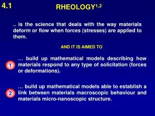
4.1 AND IT IS AIMED TO … build up mathematical models describing how materials respond to any type of solicitation (forces or deformations). 1 … build up mathematical models able to establish a link between materials macroscopic behaviour and materials micro-nanoscopic structure. 2 RHEOLOGY1,2 .. is the science that deals with the way materials deform or flow when forces (stresses) are applied to them.
4.2 A cross section area STRESS F h F S A cross section area F h NORMAL STRESS (N/M2 = Pa) SHEAR STRESS (N/M2 = Pa)
A cross section area F h L0 L F S h F LINEAR STRAIN SHEAR STRAIN HENCKY STRAIN DEFORMATION
4.3 HOOKE’s Law (small deformations) Normal stress Shear stress Incompressible materials E = 3G [SOLID MATERIAL] E = Young modulus (Pa) G = shear modulus (Pa) RHEOLOGICAL PROPERTIES A - ELASTICITY “ A material is perfectly elastic if it returns to its original shape once the deforming stress is removed”
B - VISCOSITY “ This property expresses the flowing (continuous deformation) resistance of a material (liquid) ” Very often VISCOSITY and DENSITY are used as synonyms but this is WRONG! EXAMPLE: at T = 25°C and P = 1 atm HONEY is a fluid showing high viscosity (~ 19 Pa*s) and low density (~1400 Kg/M3) MERCURY is a fluid showing low viscosity (~ 0.002 Pa*s) and high density (13579 Kg/M3) WATER: viscosity 0.001 Pa*s, density 1000 Kg/m3
NEWTON Law LIQUID MATERIAL Shear rate h = viscosity or dynamic viscosity (Pa*s) n = kinematic viscosity = h/density(m2/s)
On the contrary it can be “SHEAR THINNING” … or “SHEAR THICKENING” (opposite behaviour) IF h does not depend on share rate, the fluid is said NEWTONIAN WATERis the typical Newtonian fluid.
M M M M M K(T) K(T) K(T) K(T) M K(T) M K(T) Idealised polymer chain zfriction coefficient Usually h reduces with temperature Why h depends on liquid structure, shear rate and temperature?
LIQUID VISCOEALSTIC SOLID VISCOEALSTIC deformation deformation t t stress stress t t C - VISCOELASTICITY “ A material that does not instantaneously react to a solicitation (stress or deformation) is said viscoelastic”
STRESS Material behaviour depends on: ELASTIC (instantaneous) REACTION OF MOLECULAR SPRINGS 1 VISCOUS FRICTION AMONG: - CHAINS-CHAINS - CHAINS-SOLVENT MOLECULES 2 SOLVENT MOLECULES POLYMERIC CHAINS
D – TIXOTROPY - ANTITIXOTROPY A material is said TIXOTROPIC when its viscosity decreases with time being temperature and shear rate constant. A material is said ANTITIXOTROPIC when its viscosity increases with time being temperature and shear rate constant. The reasons for this behaviour is found in the temporal modification of system structure
h AT REST: structure MOTION structure break up COAL PARTICLE EXAMPLE: Water-Coal suspensions In the case of viscoelastic systems, no structure break up occurs t
4.4 .. consequently, linear viscoelasticty enables us to study the characteristics of material structure LINEAR VISCOELASTICITY THE LINEAR VISCOEALSTIC FIELD OCCURS FOR SMALL DEFORMATIONS / STRESSES THIS MEANS THAT MATERIAL STRUCTURE IS NOT ALTERED OR DAMAGED BY THE IMPOSED DEFORMATION / STRESS
Shear modulus G does not depend on the deformation extension g0 Shear stress Tensile modulus E does not depend on the deformation extension e0 Normal stress Incompressible materials MAIN RESULTS
G(t) or E(t) estimation g E(t) = 3 G(t) h solid g0 g0is instantaneously applied liquid 1) MAXWELL ELEMENT1,2
g1 g2 g3 g4 g5 h1 h2 h3 h4 h5 g0 g0is instantaneoulsy applied E(t) = 3 G(t) 2) GENERALISED MAXWELL MODEL1,2
g1 = 90 Pa g2 = 9 Pa g3 = 0.9 Pa g4 = 0.1 Pa
g1 g2 g3 g4 g5 h1 h2 h3 h4 h5 g(t) = g0sin(wt) w = 2pf f = solicitation frequency SMALL AMPLITUDE OSCILLATORY SHEAR
On the basis of the Boltzmann1 superposition principle, it can be demonstrated that the stress required to have a sinusoidal deformation g(t) is given by: t(t) = t0sin(wt+d) d(w) = phase shift t(t) = g0*[G’(w)*sin(wt) + G’’(w)*cos(wt)] g(t) = g0sin(wt) Gd= t0/g0=(G’2+G”2)0.5 G’(w) = Gd*cos(d) = storage modulus G’’(w) = Gd*sen(d) = loss modulus tg(d)=G”/G’
LIQUID G’≈ 0 G”≈ Gd SOLID G’≈ Gd G”≈ 0
g1 g2 g3 g4 g5 h1 h2 h3 h4 h5 According to the generalised Maxwell Model, G’ and G” can be expressed by: li = hi/gi g(t) = g0sin(wt)
In the linear viscoelastic field, oscillatory and relaxation tests lead to the same information: Oscillatory tests Relaxation tests
4.5 EXPERIMENTAL1
Rotating plate Gel Fixed plate SHEAR DEFORMATION/STRESS SHEAR RATE CONTROLLED SHEAR STRESS CONTROLLED
Linear viscoelastic range STRESS SWEEP TEST: constant frequency (1 Hz) G’(Pa) (elastic or storage modulus) t(t) = t0sin(wt) G’’(Pa) (loss or viscous modulus) w = 2pf
FREQUENCY SWEEP TEST: constant stress or deformation t0 = constant; 0.01 Hz ≤ f ≤ 100 Hz G’ (Pa) G’’ (Pa)
gi G’ (Pa) Fitting parameters gi, hi, n hi Black lines: model best fitting G’’ (Pa) t(t)
li+1 =10* li Np = generalised Maxwell model fitting parameters 0th Maxwell element (spring) -------> 1 fitting parameter (ge) 1st Maxwell element -------> 2 fitting parameters (g1, l1) 2nd Maxwell element ------->1 fitting parameters (g2, l2) 3rd Maxwell element -------> 1 fitting parameters (g3, l3) 4th Maxwell element -------> 1 fitting parameters (g4, l4)
4.6 Polymer Solvent Polymer Solvent ≈ Crosslinks FLORY THEORY3
SOLVENT mgH2O = msH2O D=mgH2O - msH2O = 0 D = DM + DE + DI = 0 Mixing Elastic Ions SWELLING EQUILIBRIUM
rx= crosslink density in the swollen state np= polymer volume fraction in the swollen state np0=polymer volume fraction in the crosslinking state T= absolute temperature R=universal gas constant gi = spring constant of the Maxwell ith element DE= -RTrx(np/np0)1/3
Comments The use of Flory theory for biopolymer gels, whose macromolecular characteristics, such as flexibility, are far from those exhibited by rubbers, has been repeatedly questioned. 1 However, recent results have shown that very stiff biopolymers might give rise to networks which are suitably described by a purely entropic approach. This holds when small deformations are considered, i.e. under linear stress-strain relationship (linear viscoelastic region)9. 2 G can be determined only inside the linear viscoelastic region. 3
x 4.7 x Polymeric chains x SAME CROSS-LINK DENSITY (rx) EQUIVALENT NETWORK TOPOLOGY EQUIVALENT NETWORK THEORY4 REAL NETWORK TOPOLOGY
REFERENCES • Lapasin R., Pricl S. Rheology of Industrial polysaccharides, Theory and Applications. Champan & Hall, London, 1995. • Grassi M., Grassi G. Lapasin R., Colombo I. Understanding drug release and absorption mechanisms: a physical and mathematical approach. CRC (Taylor & Francis Group), Boca Raton, 2007. • Flory P.J. Principles of polymer chemistry. Cornell University Press, Ithaca (NY), 1953. • Schurz J. Progress in Polymer Science, 1991, 16 (1),1991, 1.