Chapter 3 Single-Layer Perceptrons
Chapter 3 Single-Layer Perceptrons. 授課教師 : 張傳育 博士 (Chuan-Yu Chang Ph.D.) E-mail: chuanyu@yuntech.edu.tw Tel: (05)5342601 ext. 4337 Office: ES709. x 1 (i). Unknown Dynamic system. Output d(i). x 2 (i). x 3 (i). Adaptive Filter Problem.

Chapter 3 Single-Layer Perceptrons
E N D
Presentation Transcript
Chapter 3Single-Layer Perceptrons 授課教師: 張傳育 博士 (Chuan-Yu Chang Ph.D.) E-mail: chuanyu@yuntech.edu.tw Tel: (05)5342601 ext. 4337 Office: ES709
x1(i) Unknown Dynamic system Output d(i) x2(i) x3(i) Adaptive Filter Problem • 在動態系統(dynamic system)中,其數學特徵是未知的,在系統中我們所知道的只有一組由系統產生的labeled input-output data. • 也就是說,當一個m-dimension的輸入x(i)輸入到系統中,系統會產生對應的輸出d(i) 。 • 因此系統的外部行為可表示成 (3.1)
Adaptive Filter Problem (cont.) • 問題在於如何設計一多輸入單一輸出的模型? • The neural model operates under the influence of an algorithm that controls necessary adjustments to the synaptic weights of the neuron. • The algorithm starts from an arbitrary setting of the neuron’s synaptic weights. • Adjustments to the synaptic weights, in response to statistical variations in the system’s behavior, are made on a continuous basis. • Computations of adjustments to the synaptic weights are completed inside a time interval that is one sampling period long. • Adaptive model consists of two continuous processes • Filtering process, which involves the computation of two signals. • An output, and an error signal • Adaptive process • Automatic adjustment of the synaptic weights of the neuron in accordance with the error signal e(i).
v(i) x1(i) w1(i) y(i) x2(i) w2(i) -1 x3(i) w3(i) e(i) d(i) Adaptive Filter Problem (cont.) • The output y(i) is the same as the induced local field v(i) • Eq(3.2)可表示成向量的內積形式where • The neuron’s output y(i) is compared to the corresponding output d(i) (3.2) (3.4)
Unconstrained Optimization Techniques • 若一成本函數(cost function)E(w)對權重向量w是連續可微,則adaptive filtering algorithm的目的在於選擇一權重向量w,具有最小的成本。 • 若最佳的權重向量為w*,則須滿足 • Minimize the cost function E(w) with respect to the weight vector w. • The necessary condition for optimality iswhere gradient operator isthe gradient vector of the cost function is (3.5) (3.7) (3.8) (3.9)
Unconstrained Optimization Techniques • Local iterative descent • Starting with an initial guess denoted by w(0), generate a sequence of weight vectors w(1), w(2),…,such that the cost function E(w) is reduced at each iteration of the algorithmwhere w(n) is the old value of the weight vector and w(n+1) is its updated value. • We hope that the algorithm will eventually converge onto the optimal solution w*. (3.10)
Method of steepest Descent • The successive adjustments applied to the weight vector w are in the direction of steepest descent, that is in a direction opposite to the gradient vector • The steepest descent algorithm is formally described by • The correction of the algorithm is (3.11) (3.12) Stepsize/learning rate (3.13)
Method of steepest Descent (cont.) • 為了證明steepest descent algorithm滿足Eq(3.10)的條件,使用一個一階Taylor序列展開w(n)來近似E(w(n+1)) • 將Eq(3.13)代入上式,可得
Method of steepest Descent (cont.) • The method of steepest descent converges to the optimal solution w* slowly. • The learning-rate parameter h has a serious influence on its convergence behavior. • When h is small, the transient response of the algorithm is overdamped, the trajectory traced by w(n) follows a smooth path in the W-plane. • When h is large, the transient response of the algorithm is underdamped, the trajectory of w(n) follows a zigzagging (oscillatory) path. • When h exceeds a certain critical value, the algorithm becomes unstable.
Here F is assumed to be defined on the plane, and that its graph has a bowl shape. The blue curves are the contour lines, that is, the regions on which the value of F is constant. A red arrow originating at a point shows the direction of the negative gradient at that point. Note that the (negative) gradient at a point is perpendicular to the contour line going through that point. We see that gradient descent leads us to the bottom of the bowl, that is, to the point where the value of the function F is minimal.
Method of steepest Descent (cont.) • Newton’s method • To minimize the quadratic approximation of the cost functionE (w) around the current point w(n). • This minimization is performed at each iteration of the algorithm. • Using a second-order Taylor series expansion of the cost function around the point w(n).g(n) is the m-by-1 gradient vector of the cost function E (w) evaluated at the point w(n). • The matrix H(n) is the m-by-m Hessian matrix of E (w) . (3.14)
Method of steepest Descent (cont.) • The Hessian of E (w) is defined by • 從Eq(3.15)可知,cost function E (w) 必須可對w進行兩次微分 • 將Eq(3.14)對Dw進行微分,當下式滿足時, DE (w)改變量將會最小 • 上式可解得 • 也就是 (3.15) The Hessian H(n) has to be a positive definite matrix for all n. There is no guarantee that H(n)is positive definite at every iteration of the algorithm. (3.16)
Method of steepest Descent (cont.) • Gauss-Newton Method • Let the sum of error square • error signal e(i)是可調的權重向量w的函數。給定一工作點w(n) ,我們可將e(i)在w的相依性表示成其矩陣表示法為其中錯誤向量(error vector)表示成 (3.17) (3.18) (3.19)
Method of steepest Descent (cont.) • J(n) is the n-by-m Jacobian matrix of e(n): • The Jacobian J(n) is the transpose of the m-by-n gradient matrix ∇e(n) • The updated weight vector w(n+1) is then defined by (3.20) (3.21)
Method of steepest Descent (cont.) • Using Eq(3.19) to evaluate the squared Euclidean norm of e’(n,w), we get • 上式對w微分,並令結果為零,可得 • 可解得 • Gauss-Newton法只需要error vector e(n)的Jacobian matrix。但須確保JT(n)J(n)是非奇異矩陣(nonsingular) (3.22)
Method of steepest Descent (cont.) • There is no guarantee that this condition will always hold. • Add the diagonal matrix dI to the matrix JT(n)J(n). • The parameter d is a small positive constant. • On this basis, the Gauss-Newton method is implemented in the slightly modified form • The effect of this modification is progressively reduced as the number of iterations , n, is increased. • Eq(3.23)為底下modified cost function的解w(0)為權重向量w(i)的初始值。 (3.23) (3.24)
v(i) x1(i) w1(i) y(i) x2(i) w2(i) -1 x3(i) w3(i) e(i) d(i) Linear Least-Squares Filter • Linear Least-Squares Filter has two distinctive characteristics: • The single neuron is built in linear • The cost function E (w) used to design the filter consists of the sum of error squares. • 因此使用Eq(3.3)和Eq(3.4) ,error vector可表示成where d(n) is a n-by-1 desired response vector:and X(n) is the n-by-m data matrix: (3.25)
The pseudoinverse of the data matrixX(n) Linear Least-Squares Filter (cont.) • 將Eq(3.25)對w(n)微分可得梯度矩陣(gradient matrix) • e(n)的Jacobian為 • 將Eq(3.25)和 (3.26)代入(3.22)可得 • 因此,Eq(3.27)可改寫成 (3.26) (3.27) (3.28) (3.29)
Linear Least-Squares Filter (cont.) • Wiener Filter: • The input vector x(i) and desired response d(i) are draw from an ergodic environment. • We may then substitute long-term sample for expectations (ensemble averages) • Ergodic environment可使用二階統計來表示 • Correlation matrix of the input vector x(i), Rx. • Cross-correlation vector between the input vector x(i) and desired response d(i) , rx,d.where E denotes the statistical expectation operator. (3.30) (3.31)
Linear Least-Squares Filter (cont.) • Accordingly, we may reformulate the linear least-squares solution of Eq(3.27) asThe weight vector w0 is called the Wiener solution to the linear optimum filtering problem. • For an ergodic process, the linear least-square filter asymptotically approaches the Wiener filter as the number of observations approaches infinity. • However, the second-order statistics is not available in many important situations encountered in practice. (3.32)
Least-Mean-Square Algorithm • The LMS algorithm is based on the use of instantaneous values for the cost function其中,e(n)為時間n時的錯誤訊號 • 將E(n)對權重向量w微分可得 (3.33) (3.34)
Least-Mean-Square Algorithm (cont.) (3.35) • 因為 • 因此 • 所以Eq(3.34)可改寫成 • 上式稱為梯度向量的估計(Estimated Gradient vector)可得 • 套入Eq(3.12)的最陡坡降法,LMS可寫成。 (3.36) (3.37)
Least-Mean-Square Algorithm (cont.) • Summary of LMS Algorithm • Training Sample: • Input signal vector: x(n) • Desired response: d(n) • User-selected parameter: h • Initialization: • Set • Computation • For n=1, 2,…, compute
+ hx(n)d(n) + S z-1I - hx(n)xT(n) Least-Mean-Square Algorithm (cont.) • Signal-flow graph representation of LMS algorithm • 將Eq(3.35)和Eq(3.37)結合起來,可將LMS演算法的權重向量演化的過程表示成其中I為identity matrix • 因此,我們將 (3.38)
Convergence Considerations of the LMS Algorithm • 從控制理論我們知道一個回饋系統(feedback system)的穩定性(stability)是由回饋迴路的參數來決定。 • 從圖3.3,LMS演算法的回饋迴路中有兩個參數:learning rate h,input vector x(n) • LMS演算法的收斂準則 • Convergence in the mean square • 假設 • 連續的輸入向量x(1), x(2),…在統計上是彼此獨立的 • 在時間n,輸入向量x(n)對於前面所有樣本的disired response d(1), d(2),…d(n-1)是統計上獨立的 • 在時間n,desired response d(n)相依於x(n) • x(n)和d(n)是從Gaussian-distributed中取出 (3.41)
Convergence Considerations of the LMS Algorithm • By invoking the elements of independence theory and assuming that the learning rate parameter h is sufficiently small • The LMS is convergent in the mean square provided that h satisfies the conditionwhere lmax is the largest eigenvalue of the correlation matrix Rx. • 然而,在實際的 LMS的應用中,缺乏關於的lmax知識。為了解決此難題,可使用trace of Rx作為lmax的保守估計,則Eq(3.42)可改寫成 (3.42) (3.43)
Convergence Considerations of the LMS Algorithm • By definition, the trace of a square matrix is equal to the sum of its diagonal elements. • Each diagonal element of the correlation matrix Rx equals the mean-square value of the corresponding sensor input • 因此,Eq(3.43)可再改寫成 • 提供一個滿足上式的學習速率,LMS演算法可保證收斂到mean-square,(implies convergence of the mean) (3.44)
Virtues and Limitations of the LMS algorithm • Virtues of the LMS algorithm • Simplicity • Robust • Small model uncertainty and small disturbances can only result in small estimation errors. • Limitations of the LMS algorithm • Slow rate of convergence • Typically requires a number of iterations equal to about 10 times the dimensionality of the input space for it to reach a steady-state condition. • Sensitivity to variations in the eigenstructure of the input • The LMS algorithm is sensitive to variations in the condition number or eigenvalue defined by • When the condition number X(Rx) is high, the sensitivity of the LMS algorithm becomes acute. (3.45)
Learning Curves • Learning curve • Is a plot of the mean-square value of the estimation error, Eav(n), versus the number of iterations, n. • Rate of convergence • Define as the number of iterations, n, required for Eav(n) to decrease to some arbitrarily chosen value. • Such as 10 percent of the initial value Eav(0). • Misadjustment • How close the adaptive filter is to optimality in the mean-square error sense.
Learning Curves (cont.) • Misadjustment is defined aswhere Emin denote the minimum mean-square error produced by the Wiener filter, designed on the basis of known values of the correlation matrix Rx and cross-correlation vector rxd. • The misadjustment M of the LMS algorithm is directly proportional to the learning-rate parameter h. • The average time constant tav is inversely proportional to the learning rate parameter h. • If the learning rate parameter is reduced so as to reduce the misadjustment, then the settling time of the LMS algorithm is increased. • Careful attention must be given to the choice of the learning parameter h in the design of the LMS algorithm in order to produce a satisfactory overall performance. (3.46)
Learning-rate Annealing Schedules • LMS演算法在計算過程可以將learning –rate設定成幾種方式: • Constant • Learning-rate is time-varying (by Robbins, 1951)where c is a constant. When c is large, there is a danger of parameter blowup for small n. • Search-then-converge schedule (by Darken and Moody, 1992)
Learning-rate Annealing Schedules • Learning-rate annealing schedules
Perceptron • McCulloch-Pitts model • The perceptron consists of a linear combiner followed by a hard limiter (signum function). • The summing node of the neuronal model computes a linear combination of the inputs applied to its synapses, and also incorporates an externally applied bias. • The resulting sum is applied to a hard limiter. • The neuron produces an output equal to +1 if the hard limiter input is positive, and -1 if it is negative.
Bias, b x1 w1 v w2 y x2 j(v) wm xm Perceptron (cont.) • The synaptic weights of the perceptron are denoted by w1, w2,…,wm. • The inputs applied to the perceptron are denoted by x1, x2,…,xm. • The bias is denoted by b. • The induced local field of the neuron is (3.50)
x2 Class C1 Class C2 x1 Perceptron (cont.) • Perceptron的目的在於將外界輸入(x1, x2,…,xm)的刺激正確的分類為class C1或class C2。 • The decision rule for the classification is to assign the point represented by the inputs (x1, x2,…,xm) to class C1 if the perceptron output y is +1 and to class C2 if it is -1。 • The simplest form of the perceptron is two decision regions separated by a hyperplane defined by • The synaptic weights (w1, w2,…,wm) of the perceptron can be adapted on an iteration-by-iteration basis. (3.51)
x0=+1 w0=b x1 w1 v w2 y x2 j(v) wm xm Perceptron Convergence Theorem • 根據圖3.8(將圖3.6的bias納入固定輸入),則(m+1)-by-1的input vector和weight vector可表示成 • 因此,the induced local field of the neuron is defined as • wTx=0時,座標點(x1, x2,…,xm)會描繪一hyperplane,可將input分成兩類 (3.52) 其中w0(n)為bias b(n)
Decision Boundary Class C1 Class C1 Class C2 Class C2 Perceptron Convergence Theorem (cont.) 欲被分類的pattern必須有足夠的分離,以確保存在一hyperplane
Perceptron Convergence Theorem (cont.) • 假設perceptron的輸入變數,是由兩個可線性分離的class所組成,其中子集合X1={x1(1), x1(2),…} ,子集合X2={x2(1), x2(2),…} ,X1和 X2的聯集構成完整的training set X。 • 拿X1和 X2來訓練分類器,將會調整權重向量 w,使兩個類別C1和 C2可線性分離。也就是說存在一個權重向量w,使 (3.53)
Perceptron Convergence Theorem (cont.) • The algorithm for adapting the weight vector of the elementary perceptron is formulated as follows: • If the nth member of the training set, x(n), is correctly classified by the weight vector w(n), no correction is made to the weight vector of the perceptron. • Otherwise, the weight vector of the perceptron is updated in accordance with the rule (3.54) (3.55) X(n)應被分成C1但被錯分為C2; X(n)應被分成C2但被錯分為C1;
Perceptron Convergence Theorem (cont.) • 證明h=1時,fixed increment adaptation rule的收斂性。 • 假設initial condition w(0)=0,wT(n)x(n)<0 for n=1,2,…, and the input vector x(n) belongs to the subset X1。(也就是說,percetron錯將x(1), x(2)…分成第二類) h(n)=1,根據Eq(3.55)的第二式,可得 • 給訂初始條件w(0)=0,則w(n+1)可由逐次累加x(n)獲得 (3.56) (3.57)
共有n項 Perceptron Convergence Theorem (cont.) • 由於class C1和C2是假設可線性分離,因此存在一個解w0,對屬於X1子集合的所有輸入向量x(1),…,x(n) ,使wTx(n)>0。因此,可定義一正值 • 因此對Eq(3.57)兩側同時乘以wT0 • 因此,根據Eq(3.58)的定義我們可得 (3.58) (3.59)
Perceptron Convergence Theorem (cont.) • 根據Cauchy-Schwarz inequality,可知 • 將Eq(3.59)代入Eq(3.60)可得或 (3.60) (3.61)
Perceptron Convergence Theorem (cont.) • 實際上,Eq(3.56)可改寫成 (以k取代n) • 對Eq(3.62)兩邊同時取Euclidean平方,並展開可得 • 因為一開始假設perceptron錯將屬於 C1的向量x(k)分成C2,因此wT(n)x(n)<0 ,所以可從Eq(3.63)推得將上式移項,可得 (3.62) (3.63) (3.64)
Perceptron Convergence Theorem (cont.) • 代入初始條件w(0)=0,並將所有的不等式k=1,…,n加總,可得其中 • 在Eq(3.65)和Eq(3.61)中,n的值不能超過某個值nmax,此nmax必須同時滿足Eq(3.65)和Eq(3.61),因此 • 將上式移項整理可得 (3.65) (3.66) Perceptron必須在最多經過nmax次疊代後,停止調整synaptic weight (3.67)
Perceptron Convergence Theorem (cont.) • 因此,當h(n)=1 for all n, and w(0)=0, perceptron調整神經鍵的權重值,最多只需nmax次的迭代。 • Fixed-increment convergence theorem of the perceptron • Let the subsets of training vectors X1 and X2 be linearly separable. • Let the inputs presented to the perceptron originate from these two subsets. • The perceptron converges after some n0 iterations, in the sense thatis a solution vector for n0<=nmax
Perceptron Convergence Theorem (cont.) • Absolute error-correction procedure for adaptation of a single-layer perceptron • Each pattern is presented repeatedly to the perceptron until that pattern is classified correctly. • The use of an initial value w(0) merely results in a decrease or increase in the number of iterations required to converge, depending on how w(0) relates to the solution w0.
Perceptron Convergence Theorem (cont.) • Summary of the Perceptron Convergence Theorem • Initialization. Set w(0)=0. Then perform the following computations for time step n=1,2,… • Activation. Activate perceptron by applying continuous-valued input vector x(n) and desired response d(n) • Computation of Actual Response. Compute the actual response of the perceptron • Adaptation of Weight Vector. Update the weight vector of the perceptronwhere • Continuation: Increment time step n by one and go back to step 2.
Relation between the perceptron and Bayes Classifier for a Gaussian Environment • Bayes Classifier • To minimize the average risk R. • For a two-class problem, the average risk is defined aspi: a priori probability that the observation vector x is drawn from subspace Xicij: cost of deciding in favor of class Ci represented by subspace Xi when class Cj is true. • fx(x|Ci): conditional probability density function of the random vector X Correct decision (3.72) Incorrect decision
Relation between the perceptron and Bayes Classifier for a Gaussian Environment (cont.) • 由於每個observation vector x需被分成C1或C2中的一類,因此 • 因此,Eq(3.72)可改寫成where c11<c21 and c22<c12, we observe that fact that (3.73) (3.74) (3.75)