Chapter 2 Single Layer Feedforward Networks

1. Chapter 2 Single Layer Feedforward Networks

2. Perceptrons • By Rosenblatt (1962) • For modeling visual perception (retina) • A feedforward network of three layers of units: Sensory, Association, andResponse • Learning occurs only on weights from A units to R units (weights from S units to A units are fixed). • Each R unit receives inputs from n A units • For a given training sample s:t, change weights between A and R only if the computed output y is different from the target output t (error driven) wAR wSA R A S

3. Perceptrons • A simple perceptron • Structure: • Sing output node with threshold function • n input nodes with weights wi, i = 1 – n • To classify input patterns into one of the two classes (depending on whether output = 0 or 1) • Example: input patterns: (x1, x2) • Two groups of input patterns (0, 0) (0, 1) (1, 0) (-1, -1); (2.1, 0) (0, -2.5) (1.6, -1.6) • Can be separated by a line on the (x1, x2) plane x1 - x2 = 2 • Classification by a perceptron with w1 = 1, w2 = -1, threshold = 2

4. Perceptrons • Implement threshold by a node x0 • Constant output 1 • Weight w0 = - threshold • A common practice in NN design (-1, -1) (1.6, -1.6)

5. Perceptrons • Linear separability • A set of (2D) patterns (x1, x2) of two classes is linearly separable if there exists a line on the (x1, x2) plane • w0 + w1x1 + w2 x2 = 0 • Separates all patterns of one class from the other class • A perceptron can be built with • 3 input x0 = 1, x1, x2 with weights w0, w1, w2 • n dimensional patterns (x1,…, xn) • Hyperplane w0 + w1x1 + w2 x2 +…+ wn xn = 0 dividing the space into two regions • Can we get the weights from a set of sample patterns? • If the problem is linearly separable, then YES (by perceptron learning)

6. x o • Examples of linearly separable classes - Logical AND function patterns (bipolar) decision boundary x1 x2 output w1 = 1 -1 -1 -1 w2 = 1 -1 1 -1 w0 = -1 1 -1 -1 1 1 1 -1 + x1 + x2 = 0 - Logical OR function patterns (bipolar) decision boundary x1 x2 output w1 = 1 -1 -1 -1 w2 = 1 -1 1 1 w0 = 1 1 -1 1 1 1 1 1 + x1 + x2 = 0 o o x: class I (output = 1) o: class II (output = -1) x x o x x: class I (output = 1) o: class II (output = -1)

7. Perceptron Learning • The network • Input vector ij (including threshold input = 1) • Weight vector w = (w0, w1,…, wn ) • Output: bipolar (-1, 1) using the sign node function • Training samples • Pairs (ij , class(ij)) where class(ij) is the correct classification of ij • Training: • Update w so that all sample inputs are correctly classified (if possible) • If an input ij is misclassified by the current w class(ij) · w · ij < 0 change w to w + Δw so that (w + Δw) · ij is closer to class(ij)

8. Perceptron Learning Where η> 0 is the learning rate

9. Perceptron Learning • Justification

10. Perceptron learning convergence theorem • Informal: any problem that can be represented by a perceptron can be learned by the learning rule • Theorem: If there is a such that for all P training sample patterns , then for any start weight vector , the perceptron learning rule will converge to a weight vector such that for all p ( and may not be the same.) • Proof: reading for grad students (Sec. 2.4)

11. Perceptron Learning • Note: • It is a supervised learning (class(ij) is given for all sample input ij) • Learning occurs only when a sample input misclassified (error driven) • Termination criteria: learning stops when all samples are correctly classified • Assuming the problem is linearly separable • Assuming the learning rate (η) is sufficiently small • Choice of learning rate: • If η is too large: existing weights are overtaken by Δw = • If η is too small (≈ 0): very slow to converge • Common choice: η = 1. • Non-numeric input: • Different encoding schema ex. Color = (red, blue, green, yellow). (0, 0, 1, 0) encodes “green”

12. Perceptron Learning • Learning quality • Generalization: can a trained perceptron correctly classify patterns not included in the training samples? • Common problem for many NN learning models • Depends on the quality of training samples selected. • Also to some extent depends on the learning rate and initial weights (bad choices may cause learning too slow to converge to be practical) • How can we know the learning is ok? • Reserve a few samples for testing

13. Adaline • By Widrow and Hoff (~1960) • Adaptive linear elements for signal processing • The same architecture of perceptrons • Learning method: delta rule (another way of error driven), also called Widrow-Hoff learning rule Try to reduce the mean squared error (MSE) between the net input and the desired out put

14. Adaline • Delta rule • Let ij= (i0,j, i1,j,…, in,j ) be an input vector with desired output dj • The squared error • Its value determined by the weights wl • Modify weights by gradient descent approach •  • Change weights in the opposite direction of

15. Adaline Learning Algorithm

16. Adaline Learning • Delta rule in batch mode • Based on mean squared error over all P samples • E is again a function of w= (w0, w1,…, wn ) • the gradient of E: • Therefore

17. Adaline Learning • Notes: • Weights will be changed even if an input is classified correctly • E monotonically decreases until the system reaches a state with (local) minimum E (a small change of any wi will cause E to increase). • At a local minimum E state, , but E is not guaranteed to be zero (netj != dj) • This is why Adaline uses threshold function rather than linear function

18. o x o x x: class I (output = 1) o: class II (output = -1) Linear Separability Again • Examples of linearly inseparable classes - Logical XOR (exclusive OR)function patterns (bipolar) decision boundary x1 x2 output -1 -1 -1 -1 1 1 1 -1 1 1 1 -1 No line can separate these two classes, as can be seen from the fact that the following linear inequality system has no solution because we have w0 < 0 from (1) + (4), and w0 >= 0 from (2) + (3), which is a contradiction

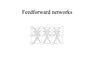
19. Y z2 z1 x1 x2 Why hidden units must be non-linear? v11 w1 • Multi-layer net with linear hidden layers is equivalent to a single layer net • Because z1 and z2 are linear unit z1 = a1* (x1*v11 + x2*v21) + b1 z1 = a2* (x1*v12 + x2*v22) + b2 • nety = z1*w1 + z2*w2 = x1*u1 + x2*u2 + b1+b2 where u1 = (a1*v11+ a2*v12)w1, u2 = (a1*v21 + a2*v22)*w2 nety is still a linear combination of x1 and x2. threshold = 0 v12 v21 w2 v22

20. 2 2 Threshold = 0 Y z2 z1 x1 x2 -2 -2 2 2 (-1, -1) (-1, -1) -1 (-1, 1) (-1, 1) 1 (1, -1) (1, -1) 1 (1, 1) (-1, -1) -1 Threshold = 1 • XOR can be solved by a more complex network with hidden units

21. Summary • Single layer nets have limited representation power (linear separability problem) • Error driven seems a good way to train a net • Multi-layer nets (or nets with non-linear hidden units) may overcome linear inseparability problem, learning methods for such nets are needed • Threshold/step output functions hinders the effort to develop learning methods for multi-layered nets