The Generalized Interpolation Material Point Method
The Generalized Interpolation Material Point Method. Compaction of a foam microstructure. Tungsten Particle Impacting sandstone. The Material Point Method (MPM). 1. 2. 3. 4. 6. 5. 1. Lagrangian material points carry all state data (position, velocity, stress, etc.).

The Generalized Interpolation Material Point Method
E N D
Presentation Transcript
Compaction of a foam microstructure
The Material Point Method (MPM) 1 2 3 4 6 5 1. Lagrangian material points carry all state data (position, velocity, stress, etc.) 2. Overlying mesh defined 3. Particle state projected to mesh, e.g.: 4. Conservation of momentum solved on mesh giving updated mesh velocity and (in principal) position. Stress at particles computed based on gradient of the mesh velocity. 5. Particle positions/velocities updated from mesh solution. 6. Discard deformed mesh. Define new mesh and repeat
Interpolation function - GIMP Cell width Particle width
Interpolation function In 2D, shape functions are formed by the products of the x and y function: Gradients involve PARTIAL derivatives, so for instance:
Steps in an MPM code Initialize particles and create (logically) a grid Project (integrate) particle data to grid (mass, velocity, etc.) Set boundary conditions on velocity Compute internal force from divergence of stress Compute acceleration on the grid (a=F/m) Integrate velocity on the grid (v* = v + a*dt) Set boundary conditions on v* and a. Compute Stress, update volume, compute dt_new Update particle position and velocity, t = t+ dt, dt = dt_new “Reset” grid and return to step 2 and repeat while t<t_final
Step 1: Particle Initialization Day 8 There are two basic methods for determining particle locations Acquire them from a file (e.g. image data) Use geometric primitives to describe geometry, and inside/outside tests to determine particle placement.
Step 1: Particle Initialization At t=0, the particles need to be initialized with the following data Position, xp Volume, vp Mass, (mp=density*volume) Velocity, Vp Stress, p = 0 Deformation Gradient (Fp =Identity) Size Lxp, Lyp (dx/PPC)
Step 2: Particle Data to Grid Compute mass and velocity on the grid, mi and vi A quick check on your work:
Step 3: Boundary Conditions For simplicity, assume that the computational domain is a rigid box. If the velocity of the rigid walls is zero, then set the velocity on those computational nodes to be zero. Also need to set the velocity on the “extra” nodes to be zero as well. Extra Nodes Domain boundary Note, for starters, you can skip this (and the other BC step) if you solve problems that stay away from the domain boundaries.
Step 4: Compute Internal Force The internal force is the volume integral of the divergence of the stress (stress is a second order tensor). The volume integral is approximated by summing the particle volumes. The divergence operation uses the gradients of the shape functions to give: Or, a bit more explicitly:
Step 5: Compute Acceleration This is basically just inverting Newton’s Second Law to get acceleration at each grid node: This is also a convenient place to include gravity:
Step 6: Integrate nodal Velocity Using basic forward Euler integration, advance the velocity at the grid nodes:
Step 7: Boundary Conditions As in Step 3, set all components of Vi* and aito zero, on both the domain boundary nodes and the “extra” nodes.
Step 8: Compute Particle Stress The first part of this step is presented in a general manner. Namely, computing the kinematic behavior at the particle level. Then a specific “constitutive model” is given for getting an elastic stress from the deformation gradient, F. First, compute the velocity gradient at each particle, based on nodal velocities: Note that this is creating a second order tensor from two vectors (first order tensors) via a dyadic product.
Step 8: Compute Particle Stress Next, we’ll use the velocity gradient tensor to update the deformation gradient F: With F in hand, one can use any number of constitutive models. A simple one is given below: Where J=det(F) and and and material specific properties.
Step 8: Compute Particle Stress Finally, update the particle volume according to: And compute a new timestep size that will satisfy the CFL stability condition:
Step 9: Update Particle State Update particle velocity according to: Lastly, update the time:
Step 10: Return to Step 2 Repeat steps 2 through 9 until the time reaches the desired simulation time.
A first Simulation Consider replicating the results from Section 7.3 of Sulsky, Chen and Schreyer, 1995. There, two cylinder of diameter (approximately) 0.5 are given initial velocities towards each other, and they collide and bounce away. Properties given are: Density = 1000 E = 1000 Poisson’s ratio = 0.3 Velocity = ( 0.1, 0.1) and (-0.1, -0.1) These values of E and Poisson’s ratio correspond to: = 577 = 385 V=(-0.1, -0.1) V=(0.1, 0.1)
A first Simulation Energy plots such as that shown in Figure 5a can be obtained by summing up the kinetic energy of the particles: KE = 0.5 *mp*vp2 The strain energy is a little more complicated. It is easiest to compute during the stress calculation, and is given by: SE = 0.5**(ln(J))-*ln(J)+0.5**(trace(FTF-3)) Again, J in this equation is the determinant of F.