Download
1 / 28
360 likes | 679 Vues
3D Simulation of particle motion in lid-driven cavity flow by MRT LBM . Arman Safdari. Ludwig Eduard Boltzmann. Born in Vienna 1844 University of Vienna 1863 Ph.D. at 22 University of Graz 1869 Died September 5, 1906. Lattice Boltzmann aim.

E N D
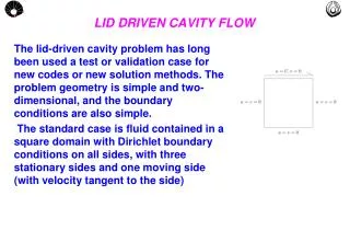
3D Simulation of particle motion in lid-driven cavity flow by MRT LBM ArmanSafdari
Ludwig Eduard Boltzmann • Born in Vienna 1844 • University of Vienna 1863 • Ph.D. at 22 • University of Graz 1869 • Died September 5, 1906
Lattice Boltzmann aim The primary goal of LB approach is to build a bridge between the microscopic and macroscopic dynamics rather than to dealt with macroscopic dynamics directly.
LBM Usage in Various Fields LBM is new & has been mostly confined to physics literature, until recently. 1
Phase Separation Streamlines LBM Capabilities Single Component Multiphase Single Phase (No Interaction) Interaction Strength Number of Components No combine Fluids/Diffusion (No Interaction) No combine Fluids Oil & water Diffusion
The Boltzmann Equation Equation describes the evolution of groups of molecules Advection terms Collision terms f : particle distribution function c : velocity of distribution function
BGK (Bhatnagar-Gross-Krook) model • most often used to solve the incompressible Navier-Stokes equations • a quasi-compressible come, in which the fluid is manufactured into adopting a slightly compressible behavior to solve the pressure equation • can also be used to simulate compressible flows at low Mach-number • It perform easily as well as its reliability
Discrete velocity model The direction of distribution function is limited to seven or nine directions 7 velocity model 9 velocity model
4 14 12 2 25 0 9 6 8 18 21 15 22 23 11 10 16 5 13 20 3 1 24 7 19 17 3D Lattice • 27 components, and 26 neighbors • 19 components, and 18 neighbors • 15 components, and 14 neighbors
BGK Boltzmann equation Equilibrium distribution function
Collision and Streaming Collision Streaming • wa are 4/9 for the rest particles (a = 0), • 1/9 for a = 1, 2, 3, 4, and • 1/36 for a = 5, 6, 7, 8. • t relaxation time • c maximum speed on lattice (1 lu/ts)
MRT (Multiple-Relaxation-Time) model • The BGK collision operator acts on the off-equilibrium part multiplying all of them with the same relaxation. But MRT can be viewed as a Multiple-Relaxation-Time model • Regularized model • better accuracy and stability are obtained by eliminating higher order, non-hydrodynamic terms from the particle populations • This model is based on the observation that the hydrodynamic limit only on the value of the first three moments (density, velocity and stress tensor) • Entropic model • The entropic lattice Boltzmann (ELB) model is similar to the BGK and the main differences are the evaluation of the equilibrium distribution function and a local modification of the relaxation time.
Boundary Condition 1-Bounce Back Bounce back is used to model solid stationary or moving boundary condition, non-slip condition, or flow-over obstacles. Type Of Bounce Back BC 2 1 3
2-Equlibrium and Non-Equlibrium Distribution Function The distribution function can be split in to two parts, equilibrium and non-equilibrium. 3- Open Boundary Condition The extrapolation method is used to find the unknown distribution functions. Second order polynomial can be used, as :
3- Periodic Boundary Condition Periodic boundary condition become necessary to apply to isolate a repeating flow conditions. For instance flow over bank of tubes. 4- Symmetry Condition Symmetry condition need to be applied along the symmetry line.
Convection by LBM This represents the mixing that would occur when saltwater is sitting on top of freshwater. CMWR 2004
Convection by LBM This is a fun simulation of heat rising from below causing convection currents. CMWR 2004
Advantages of Lattice Boltzmann Method • Macroscopic continuum equation, Navier Stoke, the LBM is based on microscopic model. LBM does not need to consider explicitly the distribution of pressure on interfaces of refined grids since the implicitly is included in the computational scheme. • The lattice Boltzmann method is particularly suited to simulating complex fluid flow • Represent both laminar and turbulent flow and handle complex and changing boundary conditions and geometries due to its simple algorithm. • 3D can be implemented with some modification • It is not difficult to calculate and shape of particle
Thank you I hope, this research can contribute to human development.