Understanding Continuous Distributions: Characteristics, Calculations, and Applications
Continuous distributions are essential in statistics, representing numerical variables whose values fall within defined ranges. They are described using density curves, which indicate probabilities by calculating the area under the curve. This guide explores concepts such as the uniform distribution, normal distributions, and empirical rules, detailing how to determine probabilities, means, and standard deviations using real-world examples. Whether examining sugar weights or student heights, learn how to apply these principles effectively in data analysis.

Understanding Continuous Distributions: Characteristics, Calculations, and Applications
E N D
Presentation Transcript
Distributions Continuous Distributions
Continuous random variables • Are numerical variables whose values fall within a range or interval • Are measurements • Can be described by density curves
Density curves • Is always on or above the horizontal axis • Has an area exactly equal to one underneath it • Often describes an overall distribution • Describe what proportions of the observations fall within each range of values
Can be any shape Are generic continuous distributions Probabilities are calculated by finding the area under the curve Unusual density curves
How do you find the area of a triangle? P(X < 2) =
What is the area of a line segment? P(X = 2) = 0 P(X < 2) = .25
In continuous distributions, P(X < 2) & P(X< 2) are the same answer. Hmmmm… Is this different than discrete distributions?
Shape is a trapezoid – How long are the bases? b1 = .5 b2 = .375 h = 1 P(X > 3) = P(1 < X < 3) = .5(.375+.5)(1)=.4375 .5(.125+.375)(2) =.5
P(X > 1) = .75 .5(2)(.25) = .25 (2)(.25) = .5
P(0.5 < X < 1.5) = .28125 .5(.25+.375)(.5) = .15625 (.5)(.25) = .125
Uniform Distribution • Is a continuous distribution that is evenly (or uniformly) distributed • Has a density curve in the shape of a rectangle • Probabilities are calculated by finding the area under the curve How do you find the area of a rectangle? Where: a & b are the endpoints of the uniform distribution
1/.12 4.92 4.98 5.04 • The Citrus Sugar Company packs sugar in bags labeled 5 pounds. However, the packaging isn’t perfect and the actual weights are uniformly distributed with a mean of 4.98 pounds and a range of .12 pounds. • Construct the uniform distribution above. What shape does a uniform distribution have? What is the height of this rectangle? How long is thisrectangle?
1/.12 4.92 4.98 5.04 • What is the probability that a randomly selected bag will weigh more than 4.97 pounds? P(X > 4.97) = What is the length of the shaded region? .07(1/.12) = .5833
1/.12 4.92 4.98 5.04 • Find the probability that a randomly selected bag weighs between 4.93 and 5.03 pounds. What is the length of the shaded region? P(4.93<X<5.03) = .1(1/.12) = .8333
1/35 5 40 • The time it takes for students to drive to school is evenly distributed with a minimum of 5 minutes and a range of 35 minutes. • Draw the distribution What is the height of the rectangle? Where should the rectangle end?
1/35 5 40 b) What is the probability that it takes less than 20 minutes to drive to school? P(X < 20) = (15)(1/35) = .4286
c) What is the mean and standard deviation of this distribution? m = (5 + 40)/2 = 22.5 s2 = (40 - 5)2/12 = 102.083 s = 10.104
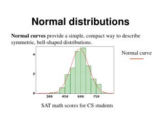
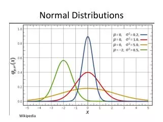
Normal Distributions • Symmetrical bell-shaped (unimodal) density curve • Above the horizontal axis • N(m, s) • The transition points occur at m+s • Probability is calculated by finding the area under the curve • As sincreases, the curve flattens & spreads out • As sdecreases, the curve gets taller and thinner How is this done mathematically?
Normal distributions occur frequently. • Length of newborn child • Height • Weight • ACT or SAT scores • Intelligence • Number of typing errors • Chemical processes
s s A B 6 Do these two normal curves have the same mean? If so, what is it? Which normal curve has a standard deviation of 3? Which normal curve has a standard deviation of 1? YES B A
Empirical Rule • Approximately 68% of the observations fall within s of m • Approximately 95% of the observations fall within 2s of m • Approximately 99.7% of the observations fall within 3s of m
68% 71 Suppose that the height of male students at NSHS is normally distributed with a mean of 71 inches and standard deviation of 2.5 inches. What is the probability that the height of a randomly selected male student is more than 73.5 inches? 1 - .68 = .32 P(X > 73.5) = 0.16
Standard Normal Density Curves Always has m = 0 & s = 1 To standardize: Must have this memorized!
Strategies for finding probabilities or proportions in normal distributions • State the probability statement • Draw a picture • Calculate the z-score • Look up the probability (proportion) in the table
The lifetime of a certain type of battery is normally distributed with a mean of 200 hours and a standard deviation of 15 hours. What proportion of these batteries can be expected to last less than 220 hours? Write the probability statement Draw & shade the curve P(X < 220) = .9082 Look up z-score in table Calculate z-score
The lifetime of a certain type of battery is normally distributed with a mean of 200 hours and a standard deviation of 15 hours. What proportion of these batteries can be expected to last more than 220 hours? P(X>220) = 1 - .9082 = .0918
The lifetime of a certain type of battery is normally distributed with a mean of 200 hours and a standard deviation of 15 hours. How long must a battery last to be in the top 5%? Look up in table 0.95 to find z- score P(X > ?) = .05 .95 .05 1.645
The heights of the female students at NSHS are normally distributed with a mean of 65 inches. What is the standard deviation of this distribution if 18.5% of the female students are shorter than 63 inches? What is the z-score for the 63? P(X < 63) = .185 -0.9 63
The heights of female teachers at NSHS are normally distributed with mean of 65.5 inches and standard deviation of 2.25 inches. The heights of male teachers are normally distributed with mean of 70 inches and standard deviation of 2.5 inches. • Describe the distribution of differences of heights (male – female) teachers. Normal distribution with m = 4.5 & s = 3.3634
4.5 • What is the probability that a randomly selected male teacher is shorter than a randomly selected female teacher? P(X<0) = .0901
Will my calculator do any of this normal stuff? • Normalpdf – use for graphing ONLY • Normalcdf – will find probability of area from lower bound to upper bound • Invnorm (inverse normal) – will find z-score for probability
Ways to Assess Normality Use graphs (dotplots, boxplots, or histograms) Normal probability (quantile) plot
Normal Scores Widths of Contact Windows Suppose we have the following observations of widths of contact windows in integrated circuit chips: 3.21 2.49 2.94 4.38 4.02 3.62 3.30 2.85 3.34 3.81 Think of selecting sample after sample of size 10 from a standard normal distribution. Then -1.539 is the average of the smallest observation from each sample & so on . . . Sketch a scatterplot by pairing the smallest normal score with the smallest observation from the data set & so on What should happen if our data set is normally distributed? To construct a normal probability plot, you can use quantities called normal score. The values of the normal scores depend on the sample size n. The normal scores when n = 10 are below: -1.539 -1.001 -0.656 -0.376 -0.123 0.123 0.376 0.656 1.001 1.539
Normal Probability (Quantile) plots The observation (x) is plotted against known normal z-scores If the points on the quantile plot lie close to a straight line, then the data is normally distributed Deviations on the quantile plot indicate nonnormal data Points far away from the plot indicate outliers Vertical stacks of points (repeated observations of the same number) is calledgranularity
Are these approximately normally distributed? 50 48 54 47 51 52 46 53 52 51 48 48 54 55 57 45 53 50 47 49 50 56 53 52 What is this called? The normal probability plot is approximately linear, so these data are approximately normal. Both the histogram & boxplot are approximately symmetrical, so these data are approximately normal.
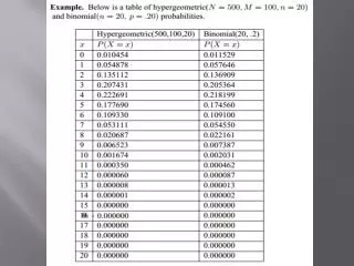
Normal Approximation to the Binomial Before widespread use of technology, binomial probability calculations were very tedious. Let’s see how statisticians estimated these calculations in the past!
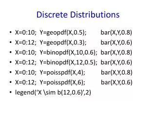
Premature babies are those born more than 3 weeks early. Newsweek (May 16, 1988) reported that 10% of the live births in the U.S. are premature. Suppose that 250 live births are randomly selected and that the number X of the “preemies” is determined. What is the probability that there are between 15 and 30 preemies, inclusive? (POD, p. 422) 1) Find this probability using the binomial distribution. 2) What is the mean and standard deviation of the above distribution? P(15<X<30) = binomialcdf(250,.1,30) – binomialcdf(250,.1,14) =.866 m = 25 & s = 4.743
Let’s graph this distribution – • Put the numbers 1-45 in L1 • In L2, use binomialpdf to find the probabilities. 3) If we were to graph a histogram for the above binomial distribution, what shape do you think it will have? 4) What do you notice about the shape? Since the probability is only 10%, we would expect the histogram to be strongly skewed right. • Overlay a normal curve on your histogram: • In Y1 = normalpdf(X,m,s)
Normal distributions can be used to estimate probabilities for binomial distributions when: 1) the probability of success is close to .5 or 2) n is sufficiently large Rule: if n is large enough, then np> 10 & n(1 –p) > 10 Why 10?
Normaldistributions extend infinitely in both directions; however,binomial distributions are between 0 and n. If we use a normal distribution to estimate a binomial distribution, we mustcut offthe tails of the normal distribution. This is OK if the mean of the normal distribution (which we use the mean of the binomial) isat least three standard deviations(3s) from 0 and from n. (BVD, p. 334)
We require: Or As binomial: Square: Simplify: Since (1 - p) < 1: And p < 1: Therefore, we say the np should be at least 10 and n (1 – p) should be at least 10.
Think about how discrete histograms are made. Each bar is centered over the discrete values. The bar for “1” actually goes from 0.5 to 1.5 & the bar for “2” goes from 1.5 to 2.5. Therefore, by adding or subtracting .5 from the discrete values, you find the actually width of the bars that you need to estimate with the normal curve. Normal distributions can be used to estimate probabilities for binomial distributions when: 1) the probability of success is close to .5 or 2) n is sufficiently large Rule: if n is large enough, then np> 10 & n(1 –p) > 10 Since a continuous distribution is used to estimate the probabilities of a discrete distribution, a continuity correction is used to make the discrete values similar to continuous values.(+.5 to discrete values) Why?
np = 250(.1) = 25 & n(1-p) = 250(.9) = 225 Yes, Ok to use normal to approximate binomial (Back to our example) Since P(preemie) = .1 which is not close to .5, is n large enough? 5) Use a normal distribution with the binomial mean and standard deviation above to estimate the probability that between 15 & 30 preemies, inclusive, are born in the 250 randomly selected babies. Binomial written as Normal(w/cont. correction) P(15 < X < 30) 6) How does the answer in question 6 compare to the answer in question 1 (Binomial answer =0.866)? P(14.5 < X < 30.5) = Normalcdf(14.5,30.5,25,4.743) = .8635


