Frequency Distributions

Frequency Distributions Quantitative Methods in HPELS 440:210

Agenda • Basic Concepts • Frequency Distribution Tables • Frequency Distribution Graphs • Percentiles and Percentile Ranks

Basic Concepts • Frequency distribution: An organized tabulation of the number of individuals located in each category on the scale of measurement • Frequency distributions can be in table or graph format • There are two elements in a frequency distribution: • The set of categories that make up the scale of measurement • The record of the frequency of individuals in each category

Basic Concepts • There are two reasons to construct frequency distributions: • Assists with choosing the appropriate test statistic (parametric vs. nonparametric) • Assists with identification of outliers

Basic Concepts • Parametric statistics require a normal distribution • Frequency distributions provide a “picture” of the data for determination of normality • If data is normal  use parametric statistic, assuming INTERVAL or RATIO • If data is non-normal  use nonparametric regardless of scale of measurement

The Normal Distribution • Characteristics: • Horizontally symmetrical • Unified mode, median and mean

Non-Normal Distributions Heavy tailed Light tailed Left skewed Right skewed

Normal Distribution • How to determine if distribution is normal: • Several methods: • Qualititative assessment • Quantitative assessment: • Kolmogorov-Smirnov • Shapiro-Wilk • Q-Q plots

Interpretation of the Q-Q Normal Plot Normal Heavy tailed Light tailed Right skew Left skew

Bottom Line: Parametric or Nonparametric? • Is the scale of measurement at least interval? • No  Nonparametric • Yes  Answer next question • Is the distribution normal? • No  Nonparametric • Yes  Parametric

Basic Concepts • The frequency distribution can assist with the identification of outliers • Outlier: An individual data point that is substantially different from the values obtained from other individuals in the same data set • Outliers can have drastic results on the test statistic

Basic Concepts • Outliers may occur naturally or maybe due to some form of error: • Measurement error  throw out • Input error  correct the error • Lack of effort or purposeful deceit on behalf of subject  throw out. • Natural occurrence  keep the data

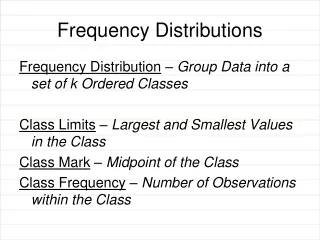
Frequency Distribution Tables • FDT contain the following information: • Scale of measurement (measurement categories) • Frequency of each point along the scale of measurement • FDT are in row/column format • Simple frequency distribution tables • Grouped frequency distribution tables

Simple Frequency Distribution Tables • Process: • List all measurement categories from lowest to highest (unless nominal) in a column (X) • List the frequency that each category occurred in the next column (f) • Example 2.1 (p 37). • Note that f = N where: • N = total number of individuals.

Simple Frequency Distribution Tables • Obtaining the X from a FDT  Process: • Create a third column called (fX) • Multiply (f) column by (X) column  product in a new (fX) column • X = fX • See Table on page 38

Simple Frequency Distribution Tables • Obtaining Proportions and Percentages: • Proportion (p): The fraction of the total group associated with each score where, • (p) = f/N • Percentage (%) = p*100 • Example 2.2 (p 37)

Grouped Frequency Distribution Tables • If the data covers a wide range of values, there are disadvantages to listing each individual score: • Cumbersome • Difficult to interpret • Grouped FDT creates groups (class intervals) of scores

Grouped Frequency Distribution Tables • There are several rules to help with the construction of grouped FDT: • Rule 1: Use ~ 10 class intervals • Too few: Lost information • Too many: Complicated • Rule 2: Width/size of each class interval should be simple • Easy to count by 2, 5 or 10. • Rule 3: The bottom score in each class interval should be a multiple of the width/size of the class interval • Example: Width/size = 5 • Each interval should start with 5, 10, 15 . . . • Rule 4: Each class interval should be the same width/size. • Example 2.3 (p 40) and Table 2.2 (p 41).

Frequency Distribution Graphs • Graphs contain same information from the frequency distribution table • Scale of measurement or measurement categories • Frequency of each category

Frequency Distribution Graphs • Format is different: • Scale of measurement is located along the horizontal x-axis (abscissa) • Values should increase from left to right. • Frequency is along the vertical y-axis (ordinate) • Values should increase from bottom to top.

Frequency Distribution Graphs • Generally speaking: • The point where the two axes intersect should have a value of zero • The height (y-axis) of the graph should be approximately 2/3 to 3/4 of its length (x-axis) • Figure 2.2 (p 44)

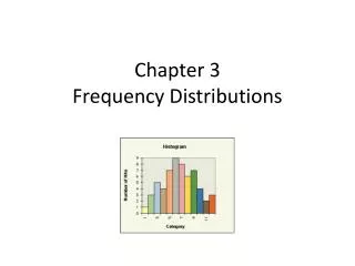
Frequency Distribution Graphs • There are several types of FDG: • Histograms (Interval/Ratio) • Polygons (Interval/Ratio) • Stem and leaf displays (Interval/Ratio) • Bar graphs (Nominal/Ordinal)

FDG: Histograms (I/R) • Process: • List the numerical scores along the x-axis • Draw a bar above each X value so that: • Height: Corresponds to the frequency • Width: Extends to the real limits of the value • Real limits: • Upper and lower • Separate adjacent scores along a number line • Example  The real limits of 150 • Lower limit = 149.5 • Upper limit = 150.5 • Figure 1.7 (p 19)

FDG: Histograms (I/R) • Bars should be in contact with each other • Extend to real limits • Figure 2.2a (p 44)

FDG: Histograms (I/R) • Variations: • Histogram from grouped frequency table • Figure 2.2b (p 45) • Modified histogram • Figure 2.4 (p 45)

FDG: Polygons (I/R) • Process: • List the numerical scores along the x-axis • Place dot above scores corresponding to frequency • Connect dots with continuous line • Draw two lines from the extreme dots to the x-axis • One category below the lowest score • One category above the highest score • Figure 2.5 (p 46)

FDG: Polygons (I/R) • Variations: • Polygon from grouped data • Figure 2.6 (p 46)

FDG: Stem and Leaf Displays (I/R) • Introduction: • Simple plot designed by J.W. Tukey (1977) • Two parts: • Stem: First digit • Leaf: Last digit(s) • Table 2.3 (p 59)

FDG: Stem and Leaf Displays (I/R) • Process: • List all stems that occur (no duplicates) • List all leaves by its stem (duplicates) • Variation: • Double stems for greater detail • First of two stems associated with leaves (0-4) • Second stem with leaves (5-9) • Table 2.4 (p 60)

FDG: Bar Graph (N/O) • Process: • Same as histogram • Spaces between the bars no real limits • Figure 2.7 (p 47) • Nominal vs. Ordinal Data: • Nominal data: The order of the categories is arbitrary • Ordinal data: Logical progression of categories • Example: Dislike, mod. dislike, no opinion, mod. like, like

Percentiles and Percentile Ranks • Introduction: • Useful when comparing scores relative to other scores • Determine the relative position of scores within the data set • Rank or percentile rank: Percentage of scores at or below the particular value • Percentile: When a score is identified by its percentile rank

Percentiles and Percentile Ranks • Process: • Within simple distribution table • Create new column (cf) cumulative frequency • Count # of scores AT or BELOW the category • Interpretation: • Cumulative frequency of 20 = 20 scores fall at or below the category • Example 2.4 (p 52)

Percentiles and Percentile Ranks • Process continued: • Same table: Add new column (c%) cumulative percentage or percentile rank • Divide (cf) value by N • Intepretation: • Percentile rank of 95% = 95% of the scores fall at or below the category • Example 2.5 (p 53)

Textbook Problem Assignment • Problems: 1, 8, 16, 17, 20a, 20c, 24, 25

Frequency Distributions