3.5 WIND LOADS 3.5.1 Wind phenomenology Wind speed is experienced essentially at two different time scales:
80 likes | 219 Vues
3.5 WIND LOADS 3.5.1 Wind phenomenology Wind speed is experienced essentially at two different time scales:

3.5 WIND LOADS 3.5.1 Wind phenomenology Wind speed is experienced essentially at two different time scales:
E N D
Presentation Transcript
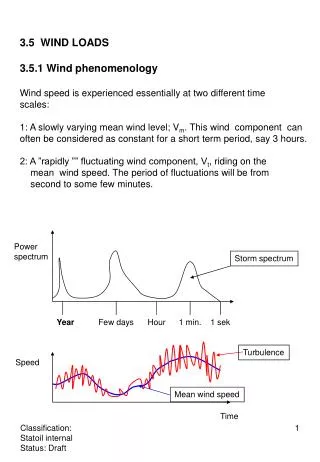
3.5 WIND LOADS3.5.1 Wind phenomenology Wind speed is experienced essentially at two different time scales: 1: A slowly varying mean wind level; Vm. This wind component can often be considered as constant for a short term period, say 3 hours. 2: A ”rapidly ”” fluctuating wind component, Vt, riding on the mean wind speed. The period of fluctuations will be from second to some few minutes. Powerspectrum Storm spectrum Year Few days Hour 1 min. 1 sek Turbulence Speed Mean wind speed Time
At a given point, the resulting wind speed can be written:V(t) = Vm(t) + Vt(t) The mean wind speed is typically the largest. Terrain roughness govern the ratio. The ratio between standarddeviation of Vt and Vm is called turbulence intencity. Typical turbulence intencity over ocean with storm waves is about 0.12. The wind speed varies with height, see eq(1a – 1d) in Statoil metocean report. For engineering purposes, the mean wind speed is described by a distribution function often close to a Rayleighdistribution. The mean direction is described by a probabilitymass function for direction sectors (often) of 30 deg. width. The mean wind speed corresponds to a given length of averaging. Standard meteorological averaging is 10 min.., in design the length of averaging is often taken to be 1 hour. Wind speed will increase with decreasing length of averaging.The ration between a 15sek average and a 1-hour average 10m above sea level is 1.37, see table in Statoil report for other examples. Example of a wind description for design purposes is shownby Statoil Metocean report.
For structures or structural components where the turbulentwind may cause a dynamic behaviour, the frequency spectrumfor wind speed is given by Eq. (2a and 2b) of Statoil Report orNorsok N-003. This wind spectrum is deduced from wind measurements atFrøya. The turbulent wind is not fully correlated over the size of structures. Coherence spectrum between two points are given in Statoil report or Norsok N-003. The loads on structures not exposed to dynamic behaviour can be calculated considering the wind as static:If structural dimensions are less than 50m, 3s gust should beused.If structures are larger, 15s gust can be used. For structures which are exposed to simultaneous actionsfrom wind and waves, and where the wave loading is dominating, the length of averaging of wind gust may be taken to be 1 minute. Check with coming editions of Norsok forpossible changes.
3.5.3 Wind forcesThe wind force is proportinal to the wind speed squared: F = k * (Vm + Vt)2 = Vm2 + 2VmVt + Vt2 =(ca) Vm2 +2VmVtThe mean wind gives a constant force on the structure, while the turbulent wind yields a force proportional the theturbulent wind speed. Practical problems:Offset and mooring line forces for ships and floating platforms.The natural periods of the surge, sway and yaw are oftenin the order of 1-2 minute, i.e. a period band where the wind frequncy spectrum has a considerable power density.For this sort of problem, a dynamic analysis has to be carried out involving the wind power spectrum. Wind loading on flare towers and drilling towers. A quasi-static analysis is often possible accounting for some dynamics by a proper dynamic amplification factor. The wind loading on complicated structures are determinedby means of tests in wind tunel. Remember that in all cases mentioned above, one will alsohave to include the simultaneous affect of waves.
The static wind force on a structural member or surface acting normal to the member or surface is given by:FW = ½ r C A V2 sinaC – shape coefficient, see DNV 30.5r – density of air (= 1.225 kg/m3 for dry air)A – projected area of member normal to force directiona – angle between wind and axis of the exposed member For the wind load of a plane truss, the load can be calculated by using A as the enclosed area of truss if aneffective shape parameter is used, C=Ce, and the transparancy of the truss is accounted for by multiplyingthe area with the solidity ratio f. Ce is found in DNV 30.5. If more than one member or truss are located behind eachother, shielding effect can be accounte for by multiplyingloads given above by the shielding factor, h. Values for hare given in DNV 30.5. Regarding the shape coefficicent, it is recommended that DNV 30.5 or an similar reference are consulted. NB: For structural sides not facing the wind, a considerablesuction force can occurr, see Fig. 3.14 b in kompendium,Moan (2004).
If structure or structural component can be exposed to windinduced dynamics, the variability of the wind force is to be accounted for:FW(t,z) = ½ C r A (Vm(z)2 + 2* Vm(z)*Vt(z,t)) * sin aIt is seen that load is linear with respect to wind speed (since Vt2 term is neglected). If the wind induced response is linearfunction of load, the wind response may be obtained using frequency domain analysis, i.e. the cross spectral density for the dynamic wind load is multiplied by response transferfunction in order to obtain response spectra for dynamicwind induced response. Alternatively, wind histories for a number of load points maybe simulated from wind spectrum and corresponding timehistories for the response found by solving the equation of motion in time domain. The total extreme wind induced response can be found by:F3h-max (Vm) = Fm + g * s(Vm)g – extreme value factor for 3-hour maximum dyn. responses – standard deviation of wind response under consideration
Vortex Induced Vibrations (brief introduction)Vortex shedding frequency in steady flow is given by:f = St * V/D St is the Strouhal number, V is wind speed and D is structuraldiameter. A critical velocity is defined as the velocity giving vortex shedding frequencies equal to the natural frequency of the structural member:VC = 1/St * fN * DfN – natural frequency of structural member. St is a function of the Reynolds number, Re = VD/n, wheren is the kinematic viscosity of air, (= 1.45*10-5 m2/s at 15oand standard atmospheric pressure. St is given in Fig. 7.1 in DNV 30.5. A state of quasi-resonant vibriations of a member may take place if wind velocity is in the range:K1*VC < V < K2*VC If possible, one should require: VC > 1/K1 *VmaxNot always possible and maybe unnecessary strict criterium.
3.6 Wave and Current loadsWater levels: Maximum still water level Positivestorm surge Highest astronomical tide (HAT) Mean still water level Tidalrange Lowest astronomical tide (LAT) Negativestorm surge Minimum still water level