Advanced Animation Techniques: Keyframes, IK, and Quaternions
Explore animation fundamentals like keyframes, skeletal hierarchy, and quaternion rotations. Learn dynamics, numerical integration, collision detection, and motion capture in digital puppetry. Enhance your animation skills with advanced methods.

Advanced Animation Techniques: Keyframes, IK, and Quaternions
E N D
Presentation Transcript
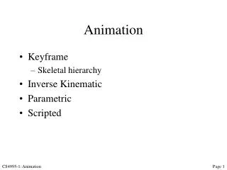
Animation • Keyframe • Skeletal hierarchy • Inverse Kinematic • Parametric • Scripted Page 1
Rotations • Euler angles – rotations about canonical axes (or in planes) • rx, ry, rz or az, el, ro • Order of rotation is important • singularities at 0o and 90o elevation • interpolations are not always “great circle” • Quaterions – rotations about a vector • ii = -1 ( = jj = kk ) • i j = k ; k i = j ; j k = i (non-commutative) • conjugate: q = w + xi + yj + zk • magnitude: ||q|| = sqrt(w2 + x2 + y2 + z2 ) • interpolations follow “great circle” • Conversion to and from Euler angles v Ref: http://www.cs.berkeley.edu/~laura/cs184/quat/quaternion.html Page 2
v Dynamics Angular dynamics • = I or = /I t+dt = t + tdt + ½t/I dt2 I = moment of inertia = torque Linear dynamics • F = ma or a = F/m at = dv/dt = d2x/dt2 vt + at dt = vt+dt = dx/dt xt + vt dt + ½ at dt2 = xt+dt • xt+dt = xt + vt dt + ½ Ft/m dt2 Page 3
1 2 v1 v2 Conservation of Momentum Angular momentum • L = I11 = I2 2 Linear momentum • p = m1v1 = m2v2 • v2 = m1v1/m2 (elastic collision) v -v Page 4
Numerical Integration dx/dt = (x, t) • Euler – xi+1= xi + h(x, t) where h = dt • Fast, but imprecise… error is O(h2) • Multi-step methods: compute intermediate results • Predictor-corrector – average slope of at t and t+1 • xpi+1 = xi + h (x, t) • xi+1 = xi + ½h ((xi, ti) + (xpi+1, ti+1)) • Runge-Kutta – 4th-order solution d1= h (xi, ti) d2 = h (ti+ ½h, xi + ½ d1) d3 = h (ti+ ½h, xi + ½ d2) d4 = h (ti+ h, xi + d3) xi+1 = xi + 1/6 (d1 + 2d2 + 2d3 + d4) Then adapt next step size (h) based on error Page 5
Collision Detection • Bounding volumes • Sphere • Axis aligned bounding box • Oriented bounding box • Bounding polygon • Intersection testing…. Backing out • Space partitioning • Projection of position over time Page 6
Motion Capture • Optical markers • Point cloud • Tracking • Marker identification • Skeletal mapping • Editing Page 7
Digital Puppetry • Real-time performance • Quick Page 8