Evaluating Finite-Rate Feedback in Multi-Antenna Systems
490 likes | 702 Vues
Evaluating Finite-Rate Feedback in Multi-Antenna Systems. Feeding Back the `Input Covariance Matrix’ Rajesh T Krishnamachari July 14, 2010. Overview of Talk. Multiple-Input Multiple-Output (MIMO) Link Channel. 1. Higher data rates than single-antenna systems.

Evaluating Finite-Rate Feedback in Multi-Antenna Systems
E N D
Presentation Transcript
Evaluating Finite-Rate Feedback in Multi-Antenna Systems Feeding Back the `Input Covariance Matrix’ Rajesh T Krishnamachari July 14, 2010
Multiple-Input Multiple-Output (MIMO) Link Channel 1 • Higher data rates than single-antenna systems. • UMTS LTE mandates Nt ≥ 2, Nr ≥ 2. 1 NOISE 2 2 + RECEIVER TRANSMITTER Nr Nt
MIMO Link Channel Equations Nt Single User Nr X Nt N1 N1 N1 Nt Nr Nr Block 1 Block 2 Block L H=H2 H=H1 H=HL i.i.d. N(0,I) Real Complex CN(0,I) Block Fading Model independent independent …
MIMO Multiple-Access Channel • … • … User 30 k30 1 • Cell has U users. • User i has kiantennas. k20 1 User 20 User 40 k40 1 • … • … Base Station k50 1 k10 User10 User 50 1 • ... • … k1 1 User 1
MIMO Basics • Assumption of Rayleigh fading : Hij ~ CN(0,1). • Input Covariance Matrix : Q = E (xxH). Computed by Telatar in 1995 for Rayleigh H.
Feedback Basics • CSIR assumption is practically sound. • Why → Tx can send pilot signals. • CSIR Capacity is • Recall → From CSITR, EH and max were exchanged. • Use feedback to convey CSI. • Why → Channel remains constant over block.
Grassmannian Quantization Single Rank Comprehensive Analysis Higher Rank Quantize Subspace on GNt, s Nt i.i.d. messages Transmit Signal
Idea of Input Covariance Feedback Feedback Rates Circuit Complexity Why not feed back the Input Covariance Matrix itself ?
Water-filling Algorithm P units water Power Allocated ---> 11
Water-filling to find Qopt P units water Power Allocated ---> • Distribution of Q not known even for Rayleigh-faded H.
Rank Convergence theorem Theorem 1 For the optimal input covariance matrix, determined by water-filling, the ratio of its rank to its size converges almost surely to a deterministic function of the signal-to-noise ratio as the number of transmit and receive antennas grow to infinity with their ratio approaching a finite constant.
Block Fading Model N1 N1 N1 … Block 1 Block 2 Block L H=H1 H=H2 H=HL … N2 N2 N2 Rank changes along with H. Case One: γ=γ2 γ=γL γ=γ1 OR Rank is relatively constant. N2 Case Two: γ=γ1 γ=γ1 γ=γ1
Dual Loop Feedback Outer– Loop Control Obtain System Mode Feedback System Mode Inner – Loop Control Reconstruct Input Covariance Matrix Quantize Input Covariance Matrix CHANNEL Data Rank Matrix Index
MIMO Multiple Access Channel (MAC) • Channel Equation . • Use Iterative Water-filling to compute • Want to feedback Q using Nfbits.
Manifolds • Sum power constraint • Individual power constraint Shortened as Shortened as
Manifold Dimension Theorem 2A
Manifold Co-ordinates • View ‘svec’ as an operation extracting coordinates. Theorem 2B
Distance Metric • Use in quantization through codebooks. • Log-det metric is not suitable. • For Int and Int , • . • For ,
Manifold Volume Theorems Theorem 3
Ball Volume Theorems • Geodesic Ball • Normalized Ball Volume Theorem 4
Idea Of A Codebook • Code • Quantization Rule Q2 Q1 Q3 Q7 Q0 Q6 Q4 Q5 VORONOI CELL
The Sphere Packing Code • Constructing optimal codebook is difficult. • Capacity difference is bounded by a factor ~ Δmax . Sphere Packing
The Random Code • Generalize idea of Random Vector Quantization. • If , generate i.i.d. Qi ~ Unif (M). • Numerical construction technique found.
Random Code Distortion Theorems For sufficiently large code size K, Theorem 5A • Compare with Dai-Liu-Rider, 2008 for Grassmann manifold, Uniform distribution and Chordal distance.
Random Codes [Continued] • Fast Convergence Nt =4, Ratio ≤1.01 • Asymptotically Tight Theorem 5B • Flat Manifold case improvement • Asymptotic optimality for quantizing uniform sources: Theorem 5C Theorem 5D
Results on Coding Theoretic Bounds • When δ is sufficiently small, then there exists a code in the following manifolds of size K and minimum distance δ, such that Theorem 6A Gilbert-Varshamov Lower Bound Hamming Upper Bound • The density of this codebook is given by Theorem 6B
Theorem For P1 Q P2 Related to Hamming Bound dmin P3 Theorem 7
Intuition Behind Capacity Difference Results • Assume γ=1. • Define • If Q and Q0 are close by, Depends on system strategy chosen. Evaluate this term’s behavior w.r.t. Nf Quantization Error Theorem 8
Capacity Difference Theorem Theorem 9 When the covariance matrix to be fed back is quantized using , the expected difference in the achievable information rate between the infinite and finite rate feedback case varies with the number of feedback bits used to quantize the covariance feedback as • Beats the previous Dabbagh-Love result with a 2-line computation. • → Compute dimension of their quantization manifold.
Immediate Application of result Theorem 10 To limit the capacity drop w.r.t. the maximal CSITR value to some X bps/Hz while using the code , we would require
Capacity Difference Theorem Theorem 11 • Capacity Difference is bounded as • To limit this difference to X bps/Hz, Theorem 12
Extensions to covariance feedback analysis Trace = ρ2 Trace ≤ ρ2 Rank = s Rank ≤ s • Many other questions in report
Other forms of feedback Stiefel Quantization
Stiefel Quantization Based on a map of Seven Falls, CO Springs.
Interference Alignment Scheme Tx1 Tx2 Txk Rx1 Rx2 Rxk K-user SISO IC: CSITR dsum = K/2 [Cadambe-Jafar, 2008]
Our work on interference alignment • CSI lies on Composite Grassmann manifold. • K-user R X 1 L-taps channel, CSI lies in . • scaling is sufficient to simulate CSITR dsum performance using IA. Conjecture : If CSI lies on manifold M, then is Nf= dim (M)/2 log P scaling sufficient to attain the same dsum as the CSITR case ?
summary • Studied finite-rate feedback in MIMO link and MAC. • Feedback spaces include , , and manifolds. • Rank of input covariance matrix converged fast to a function of SNR. • Used ball volume results to bound distortion of two different codebooks. • The difference in capacity between CSITR and finite rate feedback was shown to be