Lecture: 8 Physical Layer Impairments in Optical Networks

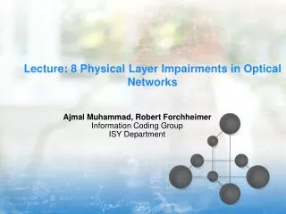
Lecture: 8 Physical Layer Impairments in Optical Networks Ajmal Muhammad, Robert Forchheimer Information Coding Group ISY Department

Outline • Introduction to Physical Layer Impairments (PLIs) • PLIs Classification • Linear and non-linear • Signal Quality Estimation • PLIs Aware Routing and Wavelength Assignment

Physical Layer Impairments Optical signals traverse the optical fibre links, passive and/or active optical components Signals encounter many impairments that affect their intensity level,as well as their temporal, spectral and polarization properties If the received signal quality is not within the receiver sensitivity threshold, the receiver may not be able to correctly detect the optical signal

Physical Layer Impairment Awareness Important for network designers and operators to know: • Various important Physical Layer Impairments (PLIs) • Their effects on lightpath (connection) feasibility • PLI analytical modeling, monitoring and mitigation techniques • Techniques to communicate PLI information to network layer and control plane protocols • How to use all these techniques to dynamically set-up and manage optically feasible lightpaths

PLIs Dependence PLIs and their significance depend on: network type, reach, type of network applications Network type: opaque (signal undergoes OEO conversion at all intermediate nodes along its path), translucent (undergoes OEO at some intermediate nodes), transparent (lightpaths are switched completely in the optical domain) Reach: Access, metro, or core/long-haul network Type of applications: Real-time, non-real time, mission-critical, etc

Maximum Transparency Length The maximum distance an optical signal can travel and be detected by a receiver without requiring OEO conversion The maximum transparency length of an optical path depends on: • The optical signal power • The fibre distance • Type of fibre and design of links (e.g., dispersion compensation) • The number of wavelengths on a single fibre • The bit-rate per wavelength • The amplification mechanism and the number of amplifiers • The number and type of switching elements through which the signals pass before reaching the egress node or before regeneration

PLIs Classification PLIs are broadly classified into two categories: linear and non-linear Optical systems that operate below a certain input power threshold exhibit a linear relationship between the input and output signal power The loss and refractive index (n) of the fibre are independent of the signal power, i.e., static in nature Important linear impairment are: fibre attenuation, component insertion loss, Amplifier Spontaneous Emission (ASE) noise, Chromatic Dispersion (CD) (or Group Velocity Dispersion (GVD)), Polarization Mode Dispersion (PMD), crosstalk and Filter Concatenation (FC)

PLIs Classification: Non-linear Non-linear impairments refer to phenomena that only occur when the signal energy propagating in a medium attains sufficiently high intensities This can be due to high launch power and/or the confinement of energy in extremely small areas, i.e., fibre core Non-linear impairments induce phase variation and introduce noise into the optical signal Important non-linear impairments are: Self Phase Modulation (SPM), Cross Phase Modulation (XPM), Four Wave Mixing (FWM)

Signal Attenuation & Insertion Loss Signal attenuation: refers to the loss of power of a signal propagating through optical fibre as distance increases Causes: material absorption, Rayleigh scattering Material absorption: impurities within fibre absorb propagating signal power, often convert the energy into heat Rayleigh scattering: photons can interact with the atoms in the fibre causing energy to be scattering in all directions If a scattered photon does not propagate in the same direction as the original signal, then signal attenuation or loss occur Insertion loss: loss of signal power resulting from the insertion of a device in an optical fibre and is usually expressed in decibels (dB)

Amplified Spontaneous Emission (ASE) Amplifiers are used to overcome fibre losses Optical noise is added by each amplifier -spontaneously emitted photons have random characteristics and manifest in the amplified signal as noise ASE noise within the signal bandwidth cannot be removed and is subject to gain from any other amplifier downstream in the optical link

Optical Signal to Noise Ratio (OSNR) Power in optical signal divided by the power in 0.1 nm of the noise spectrum Expressed in dB For amplifiers and a line system, delivering a high ONSR is good For a receiver, tolerating a low OSNR is good dB Km

Chromatic Dispersion Material Dispersion: Since refractive index (n) is a function of wavelength, different wavelengths travel at slightly different velocities. Waveguide Dispersion: Signal in the cladding travels with a different velocity than the signal in the core. This phenomenon is significant in single mode conditions. Group Velocity (Chromatic) Dispersion = Material Disp. + Waveguide Disp.

Group Velocity Dispersion

Effects of Dispersion and Attenuation

Polarizations of Fundamental Mode Two polarization states exist in the fundamental mode in a single mode fiber

Polarization Mode Dispersion (PMD) Each polarization state has a different velocity  PMD

Crosstalk Optical switches are prone to signal leakage, giving rise to crosstalk Inter-channel crosstalk: occurs between signals on adjacent channels. Can be eliminated by using narrow pass-band receivers. Intra-channel crosstalk: occurs among signals on the same wavelengths, or signals whose wavelengths fall within each other’s receiver pass-band.

Kerr Effect The refractive index (n=c/v) of optical fibre dependent on the optical signal intensity, I: n=n0 + n2I = n0 + n2 P/Aeff Where P is optical signal power, Aeff is the effective area of the fibre core cross section, n0 is the linear refractive index, n2 is the “nonlinear index coefficient” When I is large, the nonlinear component of the refractive index becomes significant, resulting in the kerr effect (change in the refractive index of a material in response to an applied electric field) Kerr effect

Self and Cross Phase Modulation (SPM & XPM ) The refractive index changes induced by the kerr effect cause phase changes in different parts of the optical pulse to travel at different speeds, resulting in new frequencies being introduced into the pulse The kerr effect inducing phase changes of a signal due to its own intensity variation is known as self phase modulation The kerr effect induces phase modulation in a signal due to intensity variations in other channels, this effect is known as cross phase modulation

Four Wave Mixing (FWM) Multiple channels at different wavelengths (frequencies) propagate down a single fibre. The signals of these channels interactto produce new signals In general, for N signal channels, the number of generated mixing product M will be: M= N2.(N-1)/2 And the generated FWM frequencies are given by: fijk=fi+fj-fk, i!=k, j!=k FWM generated by three signals FWM generated by two signals f1 & f2

Digital Processing for Impairments Compensation Encoding for Error correction Compensation for Imperfection in the modulator 22 M Gates DSP= 20 Mgates Compensation for nonlinearity DSP for compensating dispersion & shaping the spectrum Customer Traffic coming Into the chip Tx Processing

Receive Processing Undoing the polarization effects Inverting the difference b/w the transmitter laser &the receiver laser 70 T ops/s 32 nm CMOS 150 M gates 3.7 km wire (copper)

Eye Diagram Overlay the received bit stream in the time domain over a three-bit sliding window Eight 3-bit sequence Superimposition of multiple instances of the eight 3-bit binary sequences

Eye Diagram in the Presence of Signal Degradation When a received signal is degraded by optical impairments, the eye diagram becomes partially closed and distorted For ASE, this corresponds to an increase in the standard deviation of the levels For PMD and CD, this corresponds to distortions in the slope of the bit transitions and an increase in the timing jitter

Bit Error Rate (BER) and Q-factor BER: number of bits received in error as a ratio of the total number of transmitted bits idec is the signal level at the decision instant For Gaussian distributions with mean and standard deviations given by and Optimal decision threshold value Perror minimized when Q-factor

Q-factor and BER Typical BER levels range from 10-9 to 10-12, correspond to Q-factor of 6 to 8, respectively Using forward error correction (FEC), a system may tolerate up to levels of 10-3 corresponding to a Q-factor of 3

PLI-RWA Proposals When selecting a lightpath (route and wavelength), a PLI-RWA algorithm for a transparent or translucent network has to take into account the physical layer impairments as well as wavelength availability The PLIs are either considered as constraints for the RWA decisions (i.e., physical layer impairment constrained or PLIC-RWA) or the RWA decisions are made considering these impairments (i.e., physical layer impairment aware or PLIA-RWA) In PLIA-RWA, it is possible to find alternate routes considering the impairments, while in PLIC-RWA the routing decisions are constrained by PLIs

Approach 1 Compute the route and the wavelength in the traditional way and finally verify the selected lightpath considering the physical layer impairments

Approach 2 Considering the physical layer impairments values in the routing and/or wavelength assignment decisions

Approach 3 Considering the physical layer impairments values in the routing and/or wavelength assignment decisions and finally also verify the quality of the candidate lightpath PLI verification

پایگاه پاورپوینت فارسیwww.txtzoom.comبانک اطلاعات هوشمند اسلاید

Lecture: 8 Physical Layer Impairments in Optical Networks