Understanding Population Dynamics through the Leslie Matrix and Logistic Growth Models
This summary explores population models that describe equilibrium dynamics, including birth and death rates, and age-structured populations. The Leslie matrix is introduced for modeling population sizes across age classes, showing how initial age composition impacts long-term dynamics. We also discuss exponential growth, logistic models, and critical harvesting rates, culminating in insights on life expectancy and mortality rates using demographic tables. Understanding these models is vital for predicting population behavior and sustainability.

Understanding Population Dynamics through the Leslie Matrix and Logistic Growth Models
E N D
Presentation Transcript
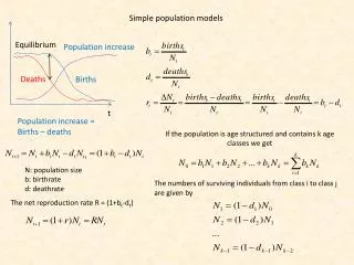
Simple populationmodels Equilibrium Populationincrease Deaths Births t Populationincrease = Births – deaths Ifthepopulationisagestructured and contains k ageclasses we get N: populationsize b: birthrate d: deathrate Thenumbers of survivingindividualsfromclass i to class j aregiven by The net reproductionrate R = (1+bt-dt)
Leslie matrix Assumeyouhave a population of organismsthatisagestructured. LetfXdenotethefecundity (rate of reproduction) atageclass x. Letsxdenotethefraction of individualsthatsurvives to thenextageclass x+1 (survivalrates). Letnxdenotethenumber of individualsatageclass x We candenotethisassumptionsin a matrix model calledthe Leslie model. We havew-1 ageclasses, wisthemaximumage of an individual. Lis a squarematrix. Numbers per ageclassat time t=1 arethedotproduct of the Leslie matrixwiththeabundancevectorNat time t
The sum of allfecunditiesgivesthenumber of newborns v n0s0givesthenumber of individualsinthe first ageclass v Nw-1sw-2givesthenumber of individualsinthelastclass v The Leslie model is a linearapproach. Itassumesstablefecundity and mortalityrates Theeffectpoftheinitialagecompositiondisappearsover time Agecompositionapproaches an equilibriumalthoughthewholepopulationmight go extinct. Population growth ordeclineisoftenexponential
An example Importantproperties: Eventuallyallageclassesgroworshrinkatthe same rate Initial growth depends on theagestructure Earlyreproductioncontributesmore to population growth thanlatereproduction Atthe long run thepopulationdies out. Reproductionratesaretoolow to counterbalancethe high mortalityrates
Doesthe Leslie approachpredict a stationary point wherepopulationabundancesdoesn’tchangeanymore? We’relooking for a vectorthatdoesn’tchangedirectionwhenmultipliedwiththe Leslie matrix. ThisvectoristheeigenvectorU of thematrix. Eigenvectorsareonlydefined for squarematrices. I: identitymatrix
Exponentialpopulation growth r=0.1 Theexponential growth model predictscontinuousincreaseordecreaseinpopulationsize. r=-0.1 Whatisifthereis an upperboundary of populationsize?
Saccharomycescerevisiae ThePearl-Verhulst model of population growth The logistic growth equation Second order differentialequation K isthecarryingcapacity (maximumpopulationsize) Maximum growth Logistic populationincrease and decrease We assumethatpopulation growth is a simplequadraticfunctionwith a maximum growth at an intermediatelevel of populationsize
Time lags The time lag model assumesthatpopulation growth mightdependet not on theprevious but on someevenearlierpopulationstates.
Intermediate growth ratesgivedampedoscillations High growth ratescangenerateincreasingpopulationcycles Low growth ratesgenerates a typical logistic growth Too high growth rateslead to extinction Certain high growth ratesproducepseudochaos High growth ratesgiveirregular but stableoscillations A simpledeterministic model isable to produceverydifferent time series and evenpseudochaos
Constantharvesting Constantharvestingrate m Whereisthestationary point whwerefishpopulationbecomesstable -4m +rK > 0 m = rK / 4 Critical harvesting rate
Life tables Alfred James Lotka (1880-1949) Vito Volterra (1860-1940) Demographicor life history tables
lt = 1 - mt-1 is the proportion of individuals that survived to interval t Cumulative mortality rate Mt Cumulative proportion surviving st is 1 - mt Mean number of individuals alive at each interval
Mean generation length isthemean period elapsingbetweethebirth of prents and thebirth of offspring Net reproduction rate of a population G = 30.2 years
The Weibull distribution is particularly used in the analysis of life expectancies and mortality rates
Thetwo parametric form B: shapeparamter T: time T: characteristic life time For t = T we get The characteristic life expectancy T istheageatwhich 63.2% of thepopulationalreadydied.
How to estimatetheparameterb and thecharacteristic life expectancy T from life historytables? We obtain b from the slope of a plot of ln[ln(1-F)] against ln(t)