Understanding Continuous Random Variables and Normal Distribution in Stochastic Models
This guide explores simple stochastic models focusing on continuous random variables, emphasizing the normal distribution and its properties. It covers the cumulative probability distribution function (CDF) and the probability density function (PDF), illustrating how these concepts apply to real-world data like students' heights and children's birth weights. Additionally, the Central Limit Theorem is examined, demonstrating its significance in the context of independent random variables with consistent mean and variance. The document also discusses fitting normal distributions to data and verifying their adherence to statistical norms.


Understanding Continuous Random Variables and Normal Distribution in Stochastic Models
E N D
Presentation Transcript
Continuous random variable X X – can take values: - < x < + Cumulative probability distribution function: PX(x) = P(X x) Probability density function:
Normal distribution X ~ normal(,), E(X)= , V(X)= 2 pdf: cpdf:
=0, =1 0.4 0.3 pdf 0.2 0.1 0 -4 -3 -2 -1 0 1 2 3 4 cpdf x
Central limit theorem Y = X1 + X2 + … +Xn Xi - independent, zero mean, equal varianceV If n is large then: ~ normal(0,1)
0.07 0.06 0.05 0.04 0.03 0.02 0.01 0 Example – students body heights Histogram of students’ body heights versus normal probability density function 160 165 170 175 180 185 190 195 200 205
9 8 7 6 5 4 3 2 1 0 Example – children birth weights Histogram of children birth weights versus normal probability density function -4 x 10 0 1000 2000 3000 4000 5000 6000
Binomial becomes normal 0.12 0.1 0.08 0.06 0.04 0.02 0 0 5 10 15 20 25 30 35 40 45 50 o – binomial(0.5,50) normal(25,3.5355)
How do we fit normal distribution to data ? Data: X1, X2, …, Xn
How do we estimate parameters of distributions using data ? • How do we verify that data follow a given distribution ?
Characteristic function X – with pdf p(x) characteristic function:
Properties Y=aX+b, a,b - constants
Characteristic function of normal distribution X ~ normal(,),
Two dimensional distributions X, Y Probability density function: p(x,y) Cumulative pdf:
Independent random variables X, Y independent pXY(x,y)=pX(x) pY(y) Convolution integral Z=X+Y pZ = pX * pY
Use of characteristic functions to prove Central Limit Theorem Y = X1 + X2 + … +Xn i=1,2…,n so: and