Option Pricing Principles and Boundaries
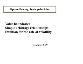
Dive into the basic principles of option pricing, value boundaries, and simple arbitrage relationships. Gain intuition about the role of volatility in option valuation through the insightful work of S. Mann in 2009.

Option Pricing Principles and Boundaries
E N D
Presentation Transcript
Option Pricing: basic principles Value boundaries Simple arbitrage relationships Intuition for the role of volatility S. Mann, 2009
Option Value Option value must be within this region Call Option Valuation "Boundaries" Intrinsic Value - Value of Immediate exercise: S - K 0 K S (asset price) Define: C[S(0),T;K] =Value of American call option with strike K, expiration date T, and current underlying asset value S(0) Result proof 1) C[0,T; K] = 0 (trivial) 2) C[S(0),T;K] >= max(0, S(0) -K) (limited liability) 3) C[S(0),T;K] <= S(0) (trivial)
“Pure time value”: K - B(0,T)K Option Value Option value must be within this region European Call lower bound (asset pays no dividend) Intrinsic value: S - K 0 KB(0,T) K S (asset price) Define: c[S(0),T;K] =Value of European call (can be exercised only at expiration) value at expiration Position cost now S(T) < K S(T) >K long call + T-bill c[S(0),T;K] + KB(0,T) K S(T) long stock S(0) S(T) S(T) position A dominates, so c[S(0),T;K] + KB(0,T) >= S(0) thus 4) c[S(0),T;K] >= Max(0, S(0) - KB(0,T)
“Pure time value”: 50 - 48.91 = $1.09 Option Value Option value must be within this region Example: Lower bound on European Call Intrinsic value: 55 - 50 0 48.91 50 55 =S(0) S (asset price) Example: S(0) =$55. K=$50. T= 3 months. 3-month simple rate=4.0%. B(0,3) = 1/(1+.04(3/12)) = 0.99. KB(0,3) = 49.50. Lower bound is S(0) - KB(0,T) = 55 – 49.50 = $5.50. What if C55 = $5.25? Value at expiration Position cash flow now S(T) <= $50 S(T) > $50 buy call - $ 5.25 0 S(T) - $50 buy bill paying K - 49.50 50 50 short stock + 55.00 -S(T) -S(T) Total + $0.25 50 - S(T) >= 0 0
American and European calls on assets without dividends 5) American call is worth at least as much as European Call C[S(0),T;K] >= c[S(0),T;K] (proof trivial) 6) American call on asset without dividends will not be exercised early. C[S(0),T;K] = c[S(0),T;K] proof: C[S(0),T;K] >= c[S(0),T;K] >= S(0) - KB(0,T) so C[S(0),T;K] >= S(0) - KB(0,T) >= S(0) - K and C[S(0),T;K] >= S(0) - K Call is: worth more alive than dead Early exercise forfeits time value 7) longer maturity cannot have negative value: for T1 > T2: C(S(0),T1;K) >= C(S(0),T2;K)
Call Option Value Option Value No-arbitrage boundary: C >= max (0, S - PV(K)) Intrinsic Value: max (0, S-K) 0 lower bound 0 K S
Low volatility asset Volatility Value : Call option Call payoff High volatility asset K S(T) (asset value)
Volatility Value : Call option Example: Equally Likely "States of World" "State of World" Expected Position Bad Avg GoodValue Stock A 24 30 36 30 Stock B 0 30 60 30 Calls w/ strike=30: Call on A: 0 0 6 2 Call on B: 0 0 30 10
K Option value must be within this region Option Value Put Option Valuation "Boundaries" Intrinsic Value - Value of Immediate exercise: K - S 0 K S (asset price) Define: P[S(0),T;K] =Value of American put option with strike K, expiration date T, and current underlying asset value S(0) Result proof 8) P[0,T; K] = K (trivial) 9) P[S(0),T;K] >= max(0, K - S(0)) (limited liability) 10) P[S(0),T;K] <= K (trivial)
KB(0,T) Option Value Option value must be within this region Negative “Pure time value”: KB(0,T) - K European Put lower bound (asset pays no dividend) Intrinsic value: K - S 0 KB(0,T) K S(0) Define: p[S(0),T;K] =Value of European put (can be exercised only at expiration) value at expiration position cost now S(T) < KS(T) >K A) long put + stock p[S(0),T;K] + S(0) K S(T) B) long T-bill KB(0,T) K K position A dominates, so p[S(0),T;K] + S(0) >= KB(0,T) thus 11) p[S(0),T;K] >= max (0, KB(0,T)- S(0))
KB(0,T) Option Value Option value must be within this region Negative “Pure time value”: KB(0,T) - K American puts and early exercise Intrinsic value: K - S 0 KB(0,T) K S(0) Define: P[S(0),T;K] =Value of American put (can be exercised at any time) 12) P[S(0),T;K] >= p[S(0),T;K] (proof trivial) However, it may be optimal to exercise a put prior to expiration (time value of money), hence American put price is not equal to European put price. Example: K=$25, S(0) = $1, six-month simple rate is 9.5%. Immediate exercise provides $24 (1+ 0.095(6/12)) = $25.14 > $25