Single-view modeling, Part 2
370 likes | 551 Vues
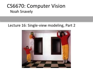
CS4670/5670: Computer Vision. Noah Snavely. Single-view modeling, Part 2. Projective geometry. Readings Mundy, J.L. and Zisserman, A., Geometric Invariance in Computer Vision, Appendix: Projective Geometry for Machine Vision, MIT Press, Cambridge, MA, 1992, (read 23.1 - 23.5, 23.10)

Single-view modeling, Part 2
E N D
Presentation Transcript
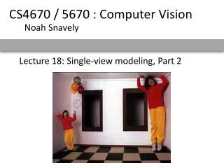
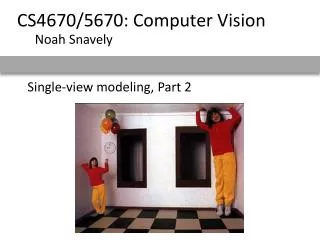
CS4670/5670: Computer Vision Noah Snavely Single-view modeling, Part 2
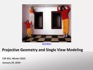
Projective geometry • Readings • Mundy, J.L. and Zisserman, A., Geometric Invariance in Computer Vision, Appendix: Projective Geometry for Machine Vision, MIT Press, Cambridge, MA, 1992, (read 23.1 - 23.5, 23.10) • available online: http://www.cs.cmu.edu/~ph/869/papers/zisser-mundy.pdf Ames Room
Announcements • Midterm to be handed in Thursday by 5pm • Please hand it back at my office, Upson 4157
v1 v2 Vanishing lines • Multiple Vanishing Points • Any set of parallel lines on the plane define a vanishing point • The union of all of these vanishing points is the horizon line • also called vanishing line • Note that different planes (can) define different vanishing lines
Vanishing lines • Multiple Vanishing Points • Any set of parallel lines on the plane define a vanishing point • The union of all of these vanishing points is the horizon line • also called vanishing line • Note that different planes (can) define different vanishing lines
Computing vanishing points V P0 D
Computing vanishing points • Properties • Pis a point at infinity, v is its projection • Depends only on line direction • Parallel lines P0 + tD, P1 + tD intersect at P V P0 D
Computing vanishing lines • Properties • l is intersection of horizontal plane through C with image plane • Compute l from two sets of parallel lines on ground plane • All points at same height as C project to l • points higher than C project above l • Provides way of comparing height of objects in the scene l v1 v2 C l ground plane
Comparing heights Vanishing Point
Measuring height 5.4 5 Camera height 4 3.3 3 2.8 2 1 How high is the camera?
Least squares version • Better to use more than two lines and compute the “closest” point of intersection • See notes by Bob Collins for one good way of doing this: • http://www-2.cs.cmu.edu/~ph/869/www/notes/vanishing.txt Computing vanishing points (from lines) v • Intersect p1q1 with p2q2 q2 q1 p2 p1
Measuring height without a ruler Z C ground plane • Compute Z from image measurements • Need more than vanishing points to do this
The cross ratio • A Projective Invariant • Something that does not change under projective transformations (including perspective projection) The cross-ratio of 4 collinear points P4 P3 P2 P1 • Can permute the point ordering • 4! = 24 different orders (but only 6 distinct values) • This is the fundamental invariant of projective geometry
scene cross ratio C image cross ratio Measuring height T (top of object) t r R (reference point) H b R B (bottom of object) vZ ground plane scene points represented as image points as
Measuring height t v H image cross ratio vz r vanishing line (horizon) t0 vx vy H R b0 b
v t1 b0 b1 Measuring height vz r t0 vanishing line (horizon) t0 vx vy m0 b • What if the point on the ground plane b0 is not known? • Here the guy is standing on the box, height of box is known • Use one side of the box to help find b0 as shown above
3D Modeling from a photograph St. Jerome in his Study, H. Steenwick
3D Modeling from a photograph Flagellation, Piero della Francesca
3D Modeling from a photograph video by Antonio Criminisi
Camera calibration • Goal: estimate the camera parameters • Version 1: solve for projection matrix • Version 2: solve for camera parameters separately • intrinsics (focal length, principle point, pixel size) • extrinsics (rotation angles, translation) • radial distortion
= = similarly, π v , π v 2 Y 3 Z Vanishing points and projection matrix = vx (X vanishing point) Not So Fast! We only know v’s up to a scale factor • Can fully specify by providing 3 reference points
Calibration using a reference object • Place a known object in the scene • identify correspondence between image and scene • compute mapping from scene to image • Issues • must know geometry very accurately • must know 3D->2D correspondence
Chromaglyphs Courtesy of Bruce Culbertson, HP Labs http://www.hpl.hp.com/personal/Bruce_Culbertson/ibr98/chromagl.htm
Estimating the projection matrix • Place a known object in the scene • identify correspondence between image and scene • compute mapping from scene to image
Direct linear calibration • Can solve for mij by linear least squares • use eigenvector trick that we used for homographies
Direct linear calibration • Advantage: • Very simple to formulate and solve • Disadvantages: • Doesn’t tell you the camera parameters • Doesn’t model radial distortion • Hard to impose constraints (e.g., known f) • Doesn’t minimize the right error function • For these reasons, nonlinear methods are preferred • Define error function E between projected 3D points and image positions • E is nonlinear function of intrinsics, extrinsics, radial distortion • Minimize E using nonlinear optimization techniques
Alternative: multi-plane calibration Images courtesy Jean-Yves Bouguet, Intel Corp. • Advantage • Only requires a plane • Don’t have to know positions/orientations • Good code available online! (including in OpenCV) • Matlab version by Jean-Yves Bouget: http://www.vision.caltech.edu/bouguetj/calib_doc/index.html • Zhengyou Zhang’s web site: http://research.microsoft.com/~zhang/Calib/
Some Related Techniques • Image-Based Modeling and Photo Editing • Mok et al., SIGGRAPH 2001 • http://graphics.csail.mit.edu/ibedit/ • Single View Modeling of Free-Form Scenes • Zhang et al., CVPR 2001 • http://grail.cs.washington.edu/projects/svm/ • Tour Into The Picture • Anjyo et al., SIGGRAPH 1997 • http://koigakubo.hitachi.co.jp/little/DL_TipE.html