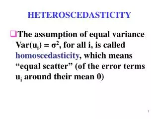
14. Scaling and Heteroscedasticity
240 likes | 399 Vues
14. Scaling and Heteroscedasticity. Using Degenerate Branches to Reveal Scaling. LIMB. Travel. Fly. BRANCH. Rail. Drive. GrndPblc. TWIG. Air. Train. Car. Bus. Scaling in Transport Modes. ----------------------------------------------------------- FIML Nested Multinomial Logit Model

14. Scaling and Heteroscedasticity
E N D
Presentation Transcript
Using Degenerate Branches to Reveal Scaling LIMB Travel Fly BRANCH Rail Drive GrndPblc TWIG Air Train Car Bus
Scaling in Transport Modes ----------------------------------------------------------- FIML Nested Multinomial Logit Model Dependent variable MODE Log likelihood function -182.42834 The model has 2 levels. Nested Logit form:IVparms=Taub|l,r,Sl|r & Fr.No normalizations imposed a priori Number of obs.= 210, skipped 0 obs --------+-------------------------------------------------- Variable| Coefficient Standard Error b/St.Er. P[|Z|>z] --------+-------------------------------------------------- |Attributes in the Utility Functions (beta) GC| .09622** .03875 2.483 .0130 TTME| -.08331*** .02697 -3.089 .0020 INVT| -.01888*** .00684 -2.760 .0058 INVC| -.10904*** .03677 -2.966 .0030 A_AIR| 4.50827*** 1.33062 3.388 .0007 A_TRAIN| 3.35580*** .90490 3.708 .0002 A_BUS| 3.11885** 1.33138 2.343 .0192 |IV parameters, tau(b|l,r),sigma(l|r),phi(r) FLY| 1.65512** .79212 2.089 .0367 RAIL| .92758*** .11822 7.846 .0000 LOCLMASS| 1.00787*** .15131 6.661 .0000 DRIVE| 1.00000 ......(Fixed Parameter)...... --------+-------------------------------------------------- NLOGIT ; Lhs=mode ; Rhs=gc,ttme,invt,invc,one ; Choices=air,train,bus,car ; Tree=Fly(Air), Rail(train), LoclMass(bus), Drive(Car) ; ivset:(drive)=[1]$
Heteroscedastic Extreme Value Model (1) +---------------------------------------------+ | Start values obtained using MNL model | | Maximum Likelihood Estimates | | Log likelihood function -184.5067 | | Dependent variable Choice | | Response data are given as ind. choice. | | Number of obs.= 210, skipped 0 bad obs. | +---------------------------------------------+ +--------+--------------+----------------+--------+--------+ |Variable| Coefficient | Standard Error |b/St.Er.|P[|Z|>z]| +--------+--------------+----------------+--------+--------+ GC | .06929537 .01743306 3.975 .0001 TTME | -.10364955 .01093815 -9.476 .0000 INVC | -.08493182 .01938251 -4.382 .0000 INVT | -.01333220 .00251698 -5.297 .0000 AASC | 5.20474275 .90521312 5.750 .0000 TASC | 4.36060457 .51066543 8.539 .0000 BASC | 3.76323447 .50625946 7.433 .0000
Heteroscedastic Extreme Value Model (2) +---------------------------------------------+ | Heteroskedastic Extreme Value Model | | Log likelihood function -182.4440 | (MNL logL was -184.5067) | Number of parameters 10 | | Restricted log likelihood -291.1218 | +---------------------------------------------+ +--------+--------------+----------------+--------+--------+ |Variable| Coefficient | Standard Error |b/St.Er.|P[|Z|>z]| +--------+--------------+----------------+--------+--------+ ---------+Attributes in the Utility Functions (beta) GC | .11903513 .06402510 1.859 .0630 TTME | -.11525581 .05721397 -2.014 .0440 INVC | -.15515877 .07928045 -1.957 .0503 INVT | -.02276939 .01122762 -2.028 .0426 AASC | 4.69411460 2.48091789 1.892 .0585 TASC | 5.15629868 2.05743764 2.506 .0122 BASC | 5.03046595 1.98259353 2.537 .0112 ---------+Scale Parameters of Extreme Value Distns Minus 1.0 s_AIR | -.57864278 .21991837 -2.631 .0085 s_TRAIN | -.45878559 .34971034 -1.312 .1896 s_BUS | .26094835 .94582863 .276 .7826 s_CAR | .000000 ......(Fixed Parameter)....... ---------+Std.Dev=pi/(theta*sqr(6)) for H.E.V. distribution. s_AIR | 3.04385384 1.58867426 1.916 .0554 s_TRAIN | 2.36976283 1.53124258 1.548 .1217 s_BUS | 1.01713111 .76294300 1.333 .1825 s_CAR | 1.28254980 ......(Fixed Parameter)....... Normalized for estimation Structural parameters
HEV Model - Elasticities +---------------------------------------------------+ | Elasticity averaged over observations.| | Attribute is INVC in choice AIR | | Effects on probabilities of all choices in model: | | * = Direct Elasticity effect of the attribute. | | Mean St.Dev | | * Choice=AIR -4.2604 1.6745 | | Choice=TRAIN 1.5828 1.9918 | | Choice=BUS 3.2158 4.4589 | | Choice=CAR 2.6644 4.0479 | | Attribute is INVC in choice TRAIN | | Choice=AIR .7306 .5171 | | * Choice=TRAIN -3.6725 4.2167 | | Choice=BUS 2.4322 2.9464 | | Choice=CAR 1.6659 1.3707 | | Attribute is INVC in choice BUS | | Choice=AIR .3698 .5522 | | Choice=TRAIN .5949 1.5410 | | * Choice=BUS -6.5309 5.0374 | | Choice=CAR 2.1039 8.8085 | | Attribute is INVC in choice CAR | | Choice=AIR .3401 .3078 | | Choice=TRAIN .4681 .4794 | | Choice=BUS 1.4723 1.6322 | | * Choice=CAR -3.5584 9.3057 | +---------------------------------------------------+ Multinomial Logit +---------------------------+ | INVC in AIR | | Mean St.Dev | | * -5.0216 2.3881 | | 2.2191 2.6025 | | 2.2191 2.6025 | | 2.2191 2.6025 | | INVC in TRAIN | | 1.0066 .8801 | | * -3.3536 2.4168 | | 1.0066 .8801 | | 1.0066 .8801 | | INVC in BUS | | .4057 .6339 | | .4057 .6339 | | * -2.4359 1.1237 | | .4057 .6339 | | INVC in CAR | | .3944 .3589 | | .3944 .3589 | | .3944 .3589 | | * -1.3888 1.2161 | +---------------------------+
Application: Shoe Brand Choice • Simulated Data: Stated Choice, 400 respondents, 8 choice situations, 3,200 observations • 3 choice/attributes + NONE • Fashion = High / Low • Quality = High / Low • Price = 25/50/75,100 coded 1,2,3,4 • Heterogeneity: Sex, Age (<25, 25-39, 40+) • Underlying data generated by a 3 class latent class process (100, 200, 100 in classes)
Multinomial Logit Baseline Values +---------------------------------------------+ | Discrete choice (multinomial logit) model | | Number of observations 3200 | | Log likelihood function -4158.503 | | Number of obs.= 3200, skipped 0 bad obs. | +---------------------------------------------+ +--------+--------------+----------------+--------+--------+ |Variable| Coefficient | Standard Error |b/St.Er.|P[|Z|>z]| +--------+--------------+----------------+--------+--------+ FASH | 1.47890473 .06776814 21.823 .0000 QUAL | 1.01372755 .06444532 15.730 .0000 PRICE | -11.8023376 .80406103 -14.678 .0000 ASC4 | .03679254 .07176387 .513 .6082
Multinomial Logit Elasticities +---------------------------------------------------+ | Elasticity averaged over observations.| | Attribute is PRICE in choice BRAND1 | | Effects on probabilities of all choices in model: | | * = Direct Elasticity effect of the attribute. | | Mean St.Dev | | * Choice=BRAND1 -.8895 .3647 | | Choice=BRAND2 .2907 .2631 | | Choice=BRAND3 .2907 .2631 | | Choice=NONE .2907 .2631 | | Attribute is PRICE in choice BRAND2 | | Choice=BRAND1 .3127 .1371 | | * Choice=BRAND2 -1.2216 .3135 | | Choice=BRAND3 .3127 .1371 | | Choice=NONE .3127 .1371 | | Attribute is PRICE in choice BRAND3 | | Choice=BRAND1 .3664 .2233 | | Choice=BRAND2 .3664 .2233 | | * Choice=BRAND3 -.7548 .3363 | | Choice=NONE .3664 .2233 | +---------------------------------------------------+
HEV Model without Heterogeneity +---------------------------------------------+ | Heteroskedastic Extreme Value Model | | Dependent variable CHOICE | | Number of observations 3200 | | Log likelihood function -4151.611 | | Response data are given as ind. choice. | +---------------------------------------------+ +--------+--------------+----------------+--------+--------+ |Variable| Coefficient | Standard Error |b/St.Er.|P[|Z|>z]| +--------+--------------+----------------+--------+--------+ ---------+Attributes in the Utility Functions (beta) FASH | 1.57473345 .31427031 5.011 .0000 QUAL | 1.09208463 .22895113 4.770 .0000 PRICE | -13.3740754 2.61275111 -5.119 .0000 ASC4 | -.01128916 .22484607 -.050 .9600 ---------+Scale Parameters of Extreme Value Distns Minus 1.0 s_BRAND1| .03779175 .22077461 .171 .8641 s_BRAND2| -.12843300 .17939207 -.716 .4740 s_BRAND3| .01149458 .22724947 .051 .9597 s_NONE | .000000 ......(Fixed Parameter)....... ---------+Std.Dev=pi/(theta*sqr(6)) for H.E.V. distribution. s_BRAND1| 1.23584505 .26290748 4.701 .0000 s_BRAND2| 1.47154471 .30288372 4.858 .0000 s_BRAND3| 1.26797496 .28487215 4.451 .0000 s_NONE | 1.28254980 ......(Fixed Parameter)....... Essentially no differences in variances across choices
Homogeneous HEV Elasticities Multinomial Logit +---------------------------------------------------+ | Attribute is PRICE in choice BRAND1 | | Mean St.Dev | | * Choice=BRAND1 -1.0585 .4526 | | Choice=BRAND2 .2801 .2573 | | Choice=BRAND3 .3270 .3004 | | Choice=NONE .3232 .2969 | | Attribute is PRICE in choice BRAND2 | | Choice=BRAND1 .3576 .1481 | | * Choice=BRAND2 -1.2122 .3142 | | Choice=BRAND3 .3466 .1426 | | Choice=NONE .3429 .1411 | | Attribute is PRICE in choice BRAND3 | | Choice=BRAND1 .4332 .2532 | | Choice=BRAND2 .3610 .2116 | | * Choice=BRAND3 -.8648 .4015 | | Choice=NONE .4156 .2436 | +---------------------------------------------------+ | Elasticity averaged over observations.| | Effects on probabilities of all choices in model: | | * = Direct Elasticity effect of the attribute. | +---------------------------------------------------+ +--------------------------+ | PRICE in choice BRAND1| | Mean St.Dev | | * -.8895 .3647 | | .2907 .2631 | | .2907 .2631 | | .2907 .2631 | | PRICE in choice BRAND2| | .3127 .1371 | | * -1.2216 .3135 | | .3127 .1371 | | .3127 .1371 | | PRICE in choice BRAND3| | .3664 .2233 | | .3664 .2233 | | * -.7548 .3363 | | .3664 .2233 | +--------------------------+
Heteroscedasticity Across Individuals +---------------------------------------------+ | Heteroskedastic Extreme Value Model | Homog-HEV MNL | Log likelihood function -4129.518[10] | -4151.611[7] -4158.503[4] +---------------------------------------------+ +--------+--------------+----------------+--------+--------+ |Variable| Coefficient | Standard Error |b/St.Er.|P[|Z|>z]| +--------+--------------+----------------+--------+--------+ ---------+Attributes in the Utility Functions (beta) FASH | 1.01640726 .20261573 5.016 .0000 QUAL | .55668491 .11604080 4.797 .0000 PRICE | -7.44758292 1.52664112 -4.878 .0000 ASC4 | .18300524 .09678571 1.891 .0586 ---------+Scale Parameters of Extreme Value Distributions s_BRAND1| .81114924 .10099174 8.032 .0000 s_BRAND2| .72713522 .08931110 8.142 .0000 s_BRAND3| .80084114 .10316939 7.762 .0000 s_NONE | 1.00000000 ......(Fixed Parameter)....... ---------+Heterogeneity in Scales of Ext.Value Distns. MALE | .21512161 .09359521 2.298 .0215 AGE25 | .79346679 .13687581 5.797 .0000 AGE39 | .38284617 .16129109 2.374 .0176
Variance Heterogeneity Elasticities Multinomial Logit +---------------------------------------------------+ | Attribute is PRICE in choice BRAND1 | | Mean St.Dev | | * Choice=BRAND1 -.8978 .5162 | | Choice=BRAND2 .2269 .2595 | | Choice=BRAND3 .2507 .2884 | | Choice=NONE .3116 .3587 | | Attribute is PRICE in choice BRAND2 | | Choice=BRAND1 .2853 .1776 | | * Choice=BRAND2 -1.0757 .5030 | | Choice=BRAND3 .2779 .1669 | | Choice=NONE .3404 .2045 | | Attribute is PRICE in choice BRAND3 | | Choice=BRAND1 .3328 .2477 | | Choice=BRAND2 .2974 .2227 | | * Choice=BRAND3 -.7458 .4468 | | Choice=NONE .4056 .3025 | +---------------------------------------------------+ +--------------------------+ | PRICE in choice BRAND1| | Mean St.Dev | | * -.8895 .3647 | | .2907 .2631 | | .2907 .2631 | | .2907 .2631 | | PRICE in choice BRAND2| | .3127 .1371 | | * -1.2216 .3135 | | .3127 .1371 | | .3127 .1371 | | PRICE in choice BRAND3| | .3664 .2233 | | .3664 .2233 | | * -.7548 .3363 | | .3664 .2233 | +--------------------------+