HETEROSCEDASTICITY
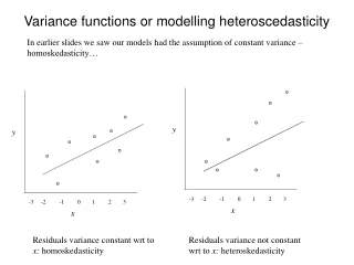
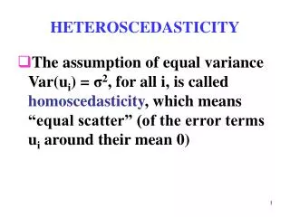
HETEROSCEDASTICITY. The assumption of equal variance Var(u i ) = σ 2 , for all i, is called homoscedasticity , which means “equal scatter” (of the error terms u i around their mean 0).

HETEROSCEDASTICITY
E N D
Presentation Transcript
HETEROSCEDASTICITY • The assumption of equal variance Var(ui) = σ2, for all i, is called homoscedasticity, which means “equal scatter” (of the error terms ui around their mean 0)
Equivalently, this means that the dispersion of the observed values of Y around the regression line is the same across all observations • If the above assumption of homoscedasticity does not hold, we have heteroscedasticity (unequal scatter)
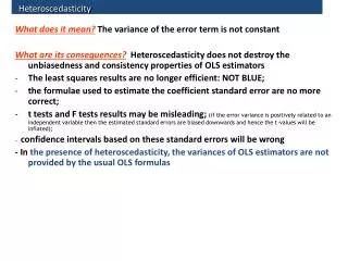
Consequences of ignoring heteroscedasticity during the OLS procedure • The estimates and forecasts based on them will still be unbiased and consistent • However, the OLS estimates are no longer the best (B in BLUE) and thus will be inefficient. Forecasts will also be inefficient
The estimated variances and covariances of the regression coefficients will be biased and inconsistent, and hence the t- and F-tests will be invalid
Testing for heteroscedasticity • 1. Before any formal tests, visually examine the model’s residuals ûi • Graph the ûi or ûi2 separately against each explanatory variable Xj, or against Ŷi, the fitted values of the dependent variable
2. The Goldfeld-Quandt test Step 1. Arrange the data from small to large values of the indp variable Xj Step 2. Run two separate regressions, one for small values of Xj and one for large values of Xj, omitting d middle observations (app. 20%), and record the residual sum of squares RSS for each regression: RSS1 for small values of Xj and RSS2 for large Xj’s.
Step 3. Calculate the ratio F = RSS2/RSS1, which has an F distribution with d.f. =[n – d – 2(k+1)]/2 both in the numerator and the denominator, where n is the total # of observations, d is the # of omitted observations, and k is the # of explanatory variables.
Step4. Reject H0: All the variances σi2 are equal (i.e., homoscedastic) if F > Fcr, where Fcr is found in the table of the F distribution for [n-d-2(k+1)]/2 d.f. and for a predetermined level of significance α, typically 5%.
Drawbacks of the the Goldfeld-Quandt test • It cannot accommodate situations where several variables jointly cause heteroscedasticity • The middle d observations are lost
3. Lagrange Multiplier (LM) tests (for large n>30) • The Breusch-Pagan test Step 1. Run the regression of ûi2 on all the explanatory variables. In our example (CN p. 37), there is only one explanatory variable, X1, therefore the model for the OLS estimation has the form: ûi2 = α0 + α1X1i + vi
Step 2. Keep the R2 from this regression. Let’s call it Rû22 Calculate either • (a) F = (Rû22/k)/[(1-Rû22)/(n-(k+1)], where k is the # of explanatory variables; the F statistic has an F distribution with d.f. = [k, n-(k+1)] Reject H0: All the variances σi2 are equal (i.e., homoscedastic) if F >Fcr
or • (b) LM = n Rû22, where LM is called the Lagrangian Multiplier (LM) statistic and has an asymptotic chi-square (χ2) distribution with d.f. = k Reject H0: All the variances σi2 are equal (i.e., homoscedastic) if LM> χcr2
Drawbacks of the Breusch-Pagan test • It has been shown to be sensitive to any violation of the normality assumption • Three other popular LM tests: the Glejser test; the Harvey-Godfrey test, and the Park test, are also sensitive to such violations (won’t be covered in this course)
One LM test, the White test, does not depend on the normality assumption; therefore it is recommended over all the other tests
The White test Step 1.The test is based on the regr. of û2 on all the explanatory varia- bles (Xj), their squares (Xj2), and all their cross products. E.g., when the model contains k = 2 explanat. variables, the test is based on an estim. of the model: û2 =β0+ β1X1 +β2X2+β3X12+β4X22 + β5X1X2 + v
Step 2. Compute the statistic χ2 = nRû22, where n is the sample size and Rû22 is the unadjusted R-squared from the OLS regression in Step 1. The statistic χ2 = nRû22, has an asymptotic chi-square (χ2) distrib. with d.f. = k, where k is the # of ALL explanatory variables in the AUXILIARY model. Reject H0: All the variances σi2 are equal (i.e., homoscedastic) if χ2 > χcr2
Estimation Procedures when H0 is rejected • 1. Heteroscedasticity with a known proportional factor • If it can be assumed that the error variance is proportional to the square of the indep. variable Xj2, we can correct for heteroscedasticity by dividing every term of the regression by X1i and then reestimating the model using the transformed variables. In the two-variable case, we will have to reestimate the following model (CN, p. 39): Yi/X1i = β0/X1i + β1 + ui/X1i
2. Heteroscedasticity consistent covariance matrix (HCCM) • As we know, the usual OLS inference is faulty in the presence of hetero-scedasticity because in this case the estimators of variances Var(bj) are biased. Therefore, new ways have been developed for estimation of hetero-scedasticity-robust variances. • The most popular is the HCCM procedure proposed by White.
The heteroscedasticity consistent covariance matrix (HCCM) procedure. • Let’s consider the model: Yi = β0 + β1X1i + β2X2i + ... + βkXki + ui • Step 1. Estimate the initial model by the OLS method. Let ûi denote the OLS residuals from the initial regression of Y on X1, X2, .., Xk
Step 2. Run the OLS regression of Xj (each time for a different j) on all other independent variables. Let ŵij denotes the ith residual from regressing Xj on all other independent variables.
Step 3. Let RSSj be the residual sum of squares from this regression: RSSj = SXjXj(1-R2). • RSSj can also be calculated as RSSj = [n-(k+1)]SER2, where SER is the standard error of regression and can easily be found in the Excel’s OLS solution.
Step 4. The heteroscedasticity-robust variance Var(bj) can be calculated as follows: Var(bj) = Σŵij2ûi2/RSSj2. • The square root of Var(bj) is called the heteroscedasticity-robust standard error for bj. • Example: CN, p. 44.
3. Feasible Generalized Least Squares (FGLS) method Step 1. Compute the residuals ûi from the OLS of the initial regression model
Step 2. Regress ûi2 against a constant term and all the explanatory variables from either the Breusch-Pagan test for heteroscedasticity (e.g., when k =2: • ûi2 = α0 + α1X1i + α2X2i + vi ) or the White test for heteroscedasticity: • ûi2 = α0 + α1X1i + α2X2i + α3X1i2 + α4X2i2 + α5X1i X2i+ vi
Step 3. Estimate the original model by OLS using the weights zi = 1/σi, where σi2 are the predicted values of the dependent variable (the ûi2) in the Breusch-Pagan (or White) model. Note: the model must be estimated without a constant term. • Such OLS procedure is called WLS (weighted least squares).
It may happen that the predicted values σi2 of the dependent variable may not be positive, so we cannot calculate the corresponding weights zi = 1/σi. If this situation arises for some observations, then we can use the original ûi2 and take their positive square roots.