Download
1 / 119
1.24k likes | 1.62k Vues
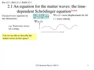
Rae §2.1, B&J §3.1, B&M §5.1. 2.1 An equation for the matter waves: the time-dependent Schr ődinger equation ***. Classical wave equation (in one dimension):. e.g. Transverse waves on a string:. x. Can we use this to describe the matter waves in free space?.

E N D
Rae §2.1, B&J §3.1, B&M §5.1 2.1 An equation for the matter waves: the time-dependent Schrődinger equation*** Classical wave equation (in one dimension): e.g. Transverse waves on a string: x Can we use this to describe the matter waves in free space? 2222 Quantum Physics 2007-8
An equation for the matter waves (2) Seem to need an equation that involves the first derivative in time, but the second derivative in space (for matter waves in free space) 2222 Quantum Physics 2007-8
An equation for the matter waves (3) For particle with potential energy V(x,t), need to modify the relationship between energy and momentum: Total energy = kinetic energy + potential energy Suggests corresponding modification to Schrődinger equation: Time-dependent Schrődinger equation 2222 Quantum Physics 2007-8 Schrődinger
The Schrődinger equation: notes • This was a plausibility argument, not a derivation. We believe the Schrődinger equation to be true not because of this argument, but because its predictions agree with experiment. • There are limits to its validity. In this form it applies to • A single particle, that is • Non-relativistic (i.e. has non-zero rest mass and velocity very much below c) • The Schrődinger equation is a partial differential equation in x and t (like classical wave equation) • The Schrődinger equation contains the complex number i. Therefore its solutions are essentially complex (unlike classical waves, where the use of complex numbers is just a mathematical convenience) 2222 Quantum Physics 2007-8
The Hamiltonian operator Can think of the RHS of the Schrődinger equation as a differential operator that represents the energy of the particle. This operator is called the Hamiltonian of the particle, and usually given the symbol Kinetic energy operator Potential energy operator Hence there is an alternative (shorthand) form for time-dependent Schrődinger equation: 2222 Quantum Physics 2007-8
Rae §2.1, B&J §2.2, B&M §5.2 2.2 The significance of the wave function*** Ψ is a complex quantity, so what can be its significance for the results of real physical measurements on a system? Remember photons: number of photons per unit volume is proportional to the electromagnetic energy per unit volume, hence to square of electromagnetic field strength. Postulate (Born interpretation): probability of finding particle in a small length δx at position x and time t is equal to Note: |Ψ(x,t)|2 is real, so probability is also real, as required. δx |Ψ|2 Total probability of finding particle between positions a and b is x Born a b 2222 Quantum Physics 2007-8
Example Suppose that at some instant of time a particle’s wavefunction is What is: (a) The probability of finding the particle between x=0.5 and x=0.5001? (b) The probability per unit length of finding the particle at x=0.6? (c) The probability of finding the particle between x=0.0 and x=0.5? 2222 Quantum Physics 2007-8
Normalization Total probability for particle to be anywhere should be one (at any time): Normalization condition • Suppose we have a solution to the Schrődinger equation that is not normalized, Then we can • Calculate the normalization integral • Re-scale the wave function as • (This works because any solution to the S.E., multiplied by a constant, remains a solution, because the equation is linear and homogeneous) Alternatively: solution to Schrödinger equation contains an arbitrary constant, which can be fixed by imposing the condition (2.7) 2222 Quantum Physics 2007-8
Normalizing a wavefunction - example 2222 Quantum Physics 2007-8
Rae §2.3, B&J §3.1 2.3 Boundary conditions for the wavefunction The wavefunction must: 1. Be a continuous and single-valued function of both x and t (in order that the probability density be uniquely defined) 2. Have a continuous first derivative (unless the potential goes to infinity) 3. Have a finite normalization integral. 2222 Quantum Physics 2007-8
Rae §2.2, B&J §3.5, B&M §5.3 2.4 Time-independent Schrődinger equation*** Suppose potential V(x,t) (and hence force on particle) is independent of time t: RHS involves only variation of Ψ with x (i.e. Hamiltonian operator does not depend on t) LHS involves only variation of Ψ with t Look for a solution in which the time and space dependence of Ψ are separated: Substitute: 2222 Quantum Physics 2007-8
Time-independent Schrődinger equation (contd) Solving the time equation: The space equation becomes: or Time-independent Schrődinger equation 2222 Quantum Physics 2007-8
Notes • In one space dimension, the time-independent Schrődinger equation is an ordinary differential equation (not a partial differential equation) • The sign of i in the time evolution is determined by the choice of the sign of i in the time-dependent Schrődinger equation • The time-independent Schrődinger equation can be thought of as an eigenvalue equation for the Hamiltonian operator: Operator × function = number × function (Compare Matrix × vector = number × vector) [See 2246] • We will consistently use uppercase Ψ(x,t) for the full wavefunction (time-dependent Schrődinger equation), and lowercase ψ(x) for the spatial part of the wavefunction when time and space have been separated (time-independent Schrődinger equation) • Probability distribution of particle is now independent of time (“stationary state”): For a stationary state we can use eitherψ(x) or Ψ(x,t) to compute probabilities; we will get the same result. 2222 Quantum Physics 2007-8
Rae §3.1, B&J §3.1, B&M §5.1 2.6 SE in three dimensions To apply the Schrődinger equation in the real (three-dimensional) world we keep the same basic structure: BUT Wavefunction and potential energy are now functions of three spatial coordinates: Kinetic energy now involves three components of momentum Interpretation of wavefunction: 2222 Quantum Physics 2007-8
Puzzle The requirement that a plane wave plus the energy-momentum relationship for free-non-relativistic particles led us to the free-particle Schrődinger equation. Can you use a similar argument to suggest an equation for free relativistic particles, with energy-momentum relationship: 2222 Quantum Physics 2007-8
3.1 A Free Particle Free particle: experiences no forces so potential energy independent of position (take as zero) Linear ODE with constant coefficients so try Time-independent Schrődinger equation: General solution: Combine with time dependence to get full wave function: 2222 Quantum Physics 2007-8
Notes • Plane wave is a solution (just as well, since our plausibility argument for the Schrődinger equation was based on this being so) • Note signs: • Sign of time term (-iωt) is fixed by sign adopted in time-dependent Schrődinger Equation • Sign of position term (±ikx) depends on propagation direction of wave • There is no restriction on the allowed energies, so there is a continuum of states 2222 Quantum Physics 2007-8
Rae §2.4, B&J §4.5, B&M §5.4 3.2 Infinite Square Well V(x) Consider a particle confined to a finite length –a<x<a by an infinitely high potential barrier x No solution in barrier region (particle would have infinite potential energy). -a a In well region: Boundary conditions: Note discontinuity in dψ/dx allowable, since potential is infinite Continuity of ψ at x=a: Continuity of ψ at x=-a: 2222 Quantum Physics 2007-8
Infinite square well (2) Add and subtract these conditions: Even solution: ψ(x)=ψ(-x) Odd solution: ψ(x)=-ψ(-x) Energy: 2222 Quantum Physics 2007-8
Infinite well – normalization and notes Normalization: Notes on the solution: • Energy quantized to particular values (characteristic of bound-state problems in quantum mechanics, where a particle is localized in a finite region of space. • Potential is even under reflection; stationary state wavefunctions may be even or odd (we say they have even or odd parity) • Compare notation in 1B23 and in books: • 1B23: well extended from x=0 to x=b • Rae and B&J: well extends from x=-a to x=+a (as here) • B&M: well extends from x=-a/2 to x=+a/2 (with corresponding differences in wavefunction) 2222 Quantum Physics 2007-8
The infinite well and the Uncertainty Principle Position uncertainty in well: Momentum uncertainty in lowest state from classical argument (agrees with fully quantum mechanical result, as we will see in §4) Compare with Uncertainty Principle: Ground state close to minimum uncertanty 2222 Quantum Physics 2007-8
V(x) III I II V0 x a -a Rae §2.4, B&J §4.6 3.3 Finite square well Now make the potential well more realistic by making the barriers a finite height V0 Region I: Region II: Region III: 2222 Quantum Physics 2007-8
Finite square well (2) Match value and derivative of wavefunction at region boundaries: Match ψ: Match dψ/dx: Add and subtract: 2222 Quantum Physics 2007-8
Finite square well (3) Divide equations: Must be satisfied simultaneously: Cannot be solved algebraically. Convenient form for graphical solution: 2222 Quantum Physics 2007-8
Graphical solution for finite well k0=3, a=1 2222 Quantum Physics 2007-8
Notes • Penetration of particle into “forbidden” region where V>E (particle cannot exist here classically) • Number of bound states depends on depth of potential well, but there is always at least one (even) state • Potential is even function, wavefunctions may be even or odd (we say they have even or odd parity) • Limit as V0→∞: 2222 Quantum Physics 2007-8
Example: the quantum well Quantum well is a “sandwich” made of two different semiconductors in which the energy of the electrons is different, and whose atomic spacings are so similar that they can be grown together without an appreciable density of defects: Material A (e.g. AlGaAs) Material B (e.g. GaAs) Electron potential energy Position Now used in many electronic devices (some transistors, diodes, solid-state lasers) Esaki Kroemer 2222 Quantum Physics 2007-8
3.4 Particle Flux Rae §9.1; B&M §5.2, B&J §3.2 In order to analyse problems involving scattering of free particles, need to understand normalization of free-particle plane-wave solutions. Conclude that if we try to normalize so that will get A=0. This problem is related to Uncertainty Principle: Position completely undefined; single particle can be anywhere from -∞ to ∞, so probability of finding it in any finite region is zero Momentum is completely defined 2222 Quantum Physics 2007-8
x a b Particle Flux (2) More generally: what is rate of change of probability that a particle exists in some region (say, between x=a and x=b)? Use time-dependent Schrődinger equation: 2222 Quantum Physics 2007-8
x a b Particle Flux (3) Integrate by parts: Flux entering at x=a - Flux leaving at x=b Interpretation: Note: a wavefunction that is real carries no current 2222 Quantum Physics 2007-8 Note: for a stationary state can use eitherψ(x) or Ψ(x,t)
Particle Flux (4) Sanity check: apply to free-particle plane wave. Makes sense: # particles passing x per unit time = # particles per unit length × velocity Wavefunction describes a “beam” of particles. 2222 Quantum Physics 2007-8
3.5 Potential Step Rae §9.1; B&J §4.3 V(x) Consider a potential which rises suddenly at x=0: V0 Case 1 x 0 Boundary condition: particles only incident from left Case 1: E<V0 (below step) x<0 x>0 2222 Quantum Physics 2007-8
Potential Step (2) Continuity of ψ at x=0: Solve for reflection and transmission: 2222 Quantum Physics 2007-8
Transmission and reflection coefficients 2222 Quantum Physics 2007-8
Potential Step (3) Case 2: E>V0(above step) Solution for x>0is now Matching conditions: Transmission and reflection coefficients: 2222 Quantum Physics 2007-8
Summary of transmission through potential step • Notes: • Some penetration of particles into forbidden region even for energies below step height (case 1, E<V0); • No transmitted particle flux, 100% reflection (case 1, E<V0); • Reflection probability does not fall to zero for energies above barrier (case 2, E>V0). • Contrast classical expectations: • 100% reflection for E<V0, with no penetration into barrier; • 100% transmission for E>V0 2222 Quantum Physics 2007-8
Rae §2.5; B&J §4.4; B&M §5.9 3.6 Rectangular Potential Barrier V(x) III I II Now consider a potential barrier of finite thickness: V0 x 0 a Boundary condition: particles only incident from left Region I: Region II: Region III: 2222 Quantum Physics 2007-8
Rectangular Barrier (2) Match value and derivative of wavefunction at region boundaries: Match ψ: Match dψ/dx: Eliminate wavefunction in central region: 2222 Quantum Physics 2007-8
Rectangular Barrier (3) Transmission and reflection coefficients: For very thick or high barrier: Non-zero transmission (“tunnelling”) through classically forbidden barrier region: 2222 Quantum Physics 2007-8
2. Alpha-decay V Distance x of α-particle from nucleus Initial α-particle energy Examples of tunnelling Tunnelling occurs in many situations in physics and astronomy: 1. Nuclear fusion (in stars and fusion reactors) V Coulomb interaction (repulsive) Incident particles Internuclear distance x Strong nuclear force (attractive) V Distance x of electron from surface Work function W Material 3. Field emission of electrons from surfaces (e.g. in plasma displays) Vacuum 2222 Quantum Physics 2007-8
Rae §2.6; B&M §5.5; B&J §4.7 3.7 Simple Harmonic Oscillator Mass m Example: particle on a spring, Hooke’s law restoring force with spring constant k: x Time-independent Schrődinger equation: Problem: still a linear differential equation but coefficients are not constant. Simplify: change variable to 2222 Quantum Physics 2007-8
Simple Harmonic Oscillator (2) Asymptotic solution in the limit of very large y: Check: Equation for H: 2222 Quantum Physics 2007-8
Simple Harmonic Oscillator (3) Must solve this ODE by the power-series method (Frobenius method); this is done as an example in 2246. • We find: • The series for H(y) must terminate in order to obtain a normalisable solution • Can make this happen after n terms for either even or odd terms in series (but not both) by choosing Hnis known as the nth Hermite polynomial. Label resulting functions of H by the values of n that we choose. 2222 Quantum Physics 2007-8
The Hermite polynomials For reference, first few Hermite polynomials are: NOTE: Hn contains yn as the highest power. Each H is either an odd or an even function, according to whether n is even or odd. 2222 Quantum Physics 2007-8
Simple Harmonic Oscillator (4) Transforming back to the original variable x, the wavefunction becomes: Probability per unit length of finding the particle is: Compare classical result: probability of finding particle in a length δx is proportional to the time δt spent in that region: For a classical particle with total energy E, velocity is given by 2222 Quantum Physics 2007-8
Notes • “Zero-point energy”: • “Quanta” of energy: • Even and odd solutions • Applies to any simple harmonic oscillator, including • Molecular vibrations • Vibrations in a solid (hence phonons) • Electromagnetic field modes (hence photons), even though this field does not obey exactly the same Schrődinger equation • You will do another, more elegant, solution method (no series or Hermite polynomials!) next year • For high-energy states, probability density peaks at classical turning points (correspondence principle) 2222 Quantum Physics 2007-8
4 Postulates of QM This section puts quantum mechanics onto a more formal mathematical footing by specifying those postulates of the theory which cannot be derived from classical physics. Main ingredients: • The wave function (to represent the state of the system); • Hermitian operators (to represent observable quantities); • A recipe for identifying the operator associated with a given observable; • A description of the measurement process, and for predicting the distribution of outcomes of a measurement; • A prescription for evolving the wavefunction in time (the time-dependent Schrődinger equation) 2222 Quantum Physics 2007-8
4.1 The wave function Postulate 4.1: There exists a wavefunction Ψthat is a continuous, square-integrable, single-valued function of the coordinates of all the particles and of time, and from which all possible predictions about the physical properties of the system can be obtained. Examples of the meaning of “The coordinates of all the particles”: For a single particle moving in one dimension: For a single particle moving in three dimensions: For two particles moving in three dimensions: The modulus squared of Ψ for any value of the coordinates is the probability density (per unit length, or volume) that the system is found with that particular coordinate value (Born interpretation). 2222 Quantum Physics 2007-8
4.2 Observables and operators Postulate 4.2.1: to each observable quantity is associated a linear, Hermitian operator (LHO). An operator is linear if and only if Examples: which of the operators defined by the following equations are linear? Note: the operators involved may or may not be differential operators (i.e. may or may not involve differentiating the wavefunction). 2222 Quantum Physics 2007-8
Hermitian operators An operator O is Hermitian if and only if: for all functions f,g vanishing at infinity. Compare the definition of a Hermitian matrix M: Analogous if we identify a matrix element with an integral: (see 3226 course for more detail…) 2222 Quantum Physics 2007-8