CS 544 Experimental Design

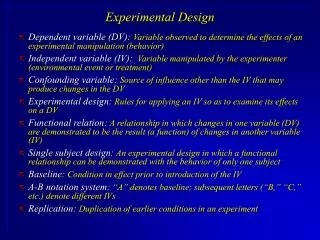
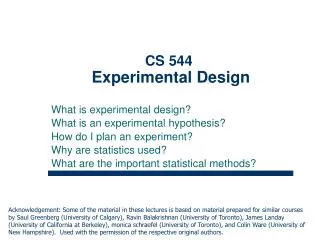
1. CS 544Experimental Design What is experimental design? What is an experimental hypothesis? How do I plan an experiment? Why are statistics used? What are the important statistical methods? Acknowledgement: Some of the material in these lectures is based on material prepared for similar courses by Saul Greenberg (University of Calgary), Ravin Balakrishnan (University of Toronto), James Landay (University of California at Berkeley), monica schraefel (University of Toronto), and Colin Ware (University of New Hampshire). Used with the permission of the respective original authors.

2. Quantitative ways to evaluate systems • Quantitative: • precise measurement, numerical values • bounds on how correct our statements are • Methods • User performance • Controlled Experiments • Statistical Analysis

3. descriptive statistics Quantitative methods 1. User performance data collection • data is collected on system use • frequency of request for on-line assistance • what did people ask for help with? • frequency of use of different parts of the system • why are parts of system unused? • number of errors and where they occurred • why does an error occur repeatedly? • time it takes to complete some operation • what tasks take longer than expected? • collect heaps of data in the hope that something interesting shows up • often difficult to sift through data unless specific aspects are targeted • as in list above

4. Quantitative methods ... 2. Controlled experiments The traditional scientific method • reductionist • clear convincing result on specific issues • In HCI: • insights into cognitive process, human performance limitations, ... • allows comparison of systems, fine-tuning of details ... Strives for • lucid and testable hypothesis (usually a causal inference – hence, inferencial statistics) • quantitative measurement • measure of confidence in results obtained replicability of experiment • control of variables and conditions • removal of experimenter bias

5. The experimental method a) Begin with a lucid, testable hypothesis • Example 1: H0: there is no difference in the number of cavities in children and teenagers using crest and no-teeth toothpaste H1: children and teenagers using crest toothpaste have fewer cavities than those who use no-teeth toothpaste

6. File Edit View Insert File New Edit New Open Open View Close Insert Close Save Save The experimental method a) Begin with a lucid, testable hypothesis • Example 2: H0: there is no difference in user performance (time and error rate) when selecting a single item from a pop-up or a pull down menu, regardless of the subject’s previous expertise in using a mouse or using the different menu types

7. The experimental method b) Explicitly state the independent variables that are to be altered Independent variables • the things you control (independent of how a subject behaves) • two different kinds: • treatment manipulated (can establish cause/effect, true experiment) • subject individual differences (can never fully establish cause/effect) in toothpaste experiment • toothpaste type: uses Crest or No-teeth toothpaste • age: <= 12 years or > 12 years in menu experiment • menu type: pop-up or pull-down • menu length: 3, 6, 9, 12, 15 • expertise: expert or novice

8. The experimental method c) Carefully choose the dependent variables that will be measured Dependent variables • variables dependent on the subject’s behaviour / reaction to the independent variable in toothpaste experiment • number of cavities • frequency of brushing in menu experiment • time to select an item • selection errors made

9. Expert Novice The experimental method d) Judiciously select and assign subjects to groups Ways of controlling subject variability • recognize classes and make them and independent variable • minimize unaccounted anomalies in subject group superstars versus poor performers • use reasonable number of subjects and random assignment

10. Now you get to do the pop-up menus. I think you will really like them... I designed them myself! The experimental method... e) Control for biasing factors • unbiased instructions + experimental protocols prepare ahead of time • double-blind experiments, ...

11. The experimental method f) Apply statistical methods to data analysis • Confidence limits: the confidence that your conclusion is correct • “The hypothesis that mouse experience makes no difference is rejected at the .05 level” (i.e., null hypothesis rejected) • means: • a 95% chance that your finding is correct • a 5% chance you are wrong g) Interpret your results • what you believe the results mean, and their implications • yes, there can be a subjective component to quantitative analysis

12. The Planning Flowchart Stage 1 Stage 2 Stage 3 Stage 4 Stage 5 Problem Planning Conduct Analysis Interpret- definition research ation feedback research define data interpretation preliminary idea variables reductions testing generalization literature review controls statistics data reporting collection apparatus hypothesis statement of testing problem procedures hypothesis select development subjects experimental design feedback

13. Statistical Analysis • What is a statistic? • a number that describes a sample • sample is a subset (hopefully representative) of the population we are interested in understanding • Statistics are calculations that tell us • mathematical attributes about our data sets (sample) • mean, amount of variance, ... • how data sets relate to each other • whether we are “sampling” from the same or different populations • the probability that our claims are correct • “statistical significance”

14. Example: Differences between means • Given: two data sets measuring a condition • eg height difference of males and females time to select an item from different menu styles ... • Question: • is the difference between the means of the data statistically significant? • Null hypothesis: • there is no difference between the two means • statistical analysis can only reject the hypothesis at a certain level of confidence • we never actually prove the hypothesis true

15. Example: mean = 4.5 3 Is there a significant difference between the means? 2 1 Condition one: 3, 4, 4, 4, 5, 5, 5, 6 0 3 4 5 6 7 Condition 1 Condition 1 3 mean = 5.5 2 1 Condition two: 4, 4, 5, 5, 6, 6, 7, 7 0 3 4 5 6 7 Condition 2 Condition 2

16. The problem with visual inspection of data • There is almost always variation in the collected data • Differences between data sets may be due to: • normal variation • eg two sets of ten tosses with different but fair dice • differences between data and means are accountable by expected variation • real differences between data • eg two sets of ten tosses with loaded dice and fair dice • differences between data and means are not accountable by expected variation

17. T-test A statistical test Allows one to say something about differences between means at a certain confidence level Null hypothesis of the T-test: • no difference exists between the means Possible results: • I am 95% sure that null hypothesis is rejected • there is probably a true difference between the means • I cannot reject the null hypothesis • the means are likely the same

18. Different types of T-tests Comparing two sets of independent observations • usually different subjects in each group (number may differ as well) Condition 1 Condition 2 S1–S20 S21–43 Paired observations • usually single group studied under separate experimental conditions • data points of one subject are treated as a pair Condition 1 Condition 2 S1–S20 S1–S20 Non-directional vs directional alternatives • non-directional (two-tailed) • no expectation that the direction of difference matters • directional (one-tailed) • Only interested if the mean of a given condition is greater than the other

19. T-tests • Assumptions of t-tests • data points of each sample are normally distributed • but t-test very robust in practice • sample variances are equal • t-test reasonably robust for differing variances • deserves consideration • individual observations of data points in sample are independent • must be adhered to • Significance level • decide upon the level before you do the test! • typically stated at the .05 or .01 level

20. Two-tailed unpaired T-test • n: number of data points in the one sample (N = n1 + n2) • SX: sum of all data points in one sample • X: mean of data points in sample • S(X2): sum of squares of data points in sample • s2: unbiased estimate of population variation • t: t ratio • df = degrees of freedom = N1 + N2 – 2 • Formulas

21. Level of significance for two-tailed test df .05 .01 1 12.706 63.657 2 4.303 9.925 3 3.182 5.841 4 2.776 4.604 5 2.571 4.032 6 2.447 3.707 7 2.365 3.499 8 2.306 3.355 9 2.262 3.250 10 2.228 3.169 11 2.201 3.106 12 2.179 3.055 13 2.160 3.012 14 2.145 2.977 15 2.131 2.947 df .05 .01 16 2.120 2.921 18 2.101 2.878 20 2.086 2.845 22 2.074 2.819 24 2.064 2.797

22. Example Calculation x1 = 3 4 4 4 5 5 5 6 Hypothesis: there is no significant difference x2 = 4 4 5 5 6 6 7 7 between the means at the .05 level Step 1. Calculating s2

23. Example Calculation Step 2. Calculating t • Step 3: Looking up critical value of t • Use table for two-tailed t-test, at p=.05, df=14 • critical value = 2.145 • because t=1.871 < 2.145, there is no significant difference • therefore, we cannot reject the null hypothesis i.e., there is no difference between the means

24. Two-tailed Unpaired T-test Condition one: 3, 4, 4, 4, 5, 5, 5, 6 Condition two: 4, 4, 5, 5, 6, 6, 7, 7 Unpaired t-test Prob. (2-tail): DF: Unpaired t Value: 14 -1.871 .0824 Group: Count: Mean: Std. Dev.: Std. Error: one 8 4.5 .926 .327 two 8 5.5 1.195 .423

25. Choice of significance levels and two types of errors • Type I error: reject the null hypothesis when it is, in fact, true ( = .05) • Type II error: accept the null hypothesis when it is, in fact, false () • Effects of levels of significance • very high confidence level (eg .0001) gives greater chance of Type II errors • very low confidence level (eg .1) gives greater chance of Type I errors • choice often depends on effects of result

26. New Open Close Close Open New Save Save Choice of significance levels and two types of errors There is no difference between Pie menus and traditional pop-up menus • Type I: extra work developing software and having people learn a new idiom for no benefit • Type II: use a less efficient (but already familiar) menu • Case 1: Redesigning a traditional GUI interface • a Type II error is preferable to a Type I error , Why? • Case 2: Designing a digital mapping application where experts perform extremely frequent menu selections • a Type I error is preferable to a Type II error, Why?

27. Other Tests: Correlation • Measures the extent to which two concepts are related • eg years of university training vs computer ownership per capita • How? • obtain the two sets of measurements • calculate correlation coefficient • +1: positively correlated • 0: no correlation (no relation) • –1: negatively correlated • Dangers • attributing causality • a correlation does not imply cause and effect • cause may be due to a third “hidden” variable related to both other variables • eg (above example) age, affluence • drawing strong conclusion from small numbers • unreliable with small groups • be wary of accepting anything more than the direction of correlation unless you have at least 40 subjects

28. Sample Study: Cigarette Consumption Crude Male death rate for lung cancer in 1950 per capita consumption of cigarettes in 1930 in various countries.

29. 10 9 8 7 6 5 4 3 2.5 3 3.5 4 4.5 5 5.5 6 6.5 7 7.5 Correlation r2 = .668 condition 1 condition 2 5 6 4 5 6 7 4 4 5 6 3 5 5 7 4 4 5 7 6 7 6 6 7 7 6 8 7 9 Condition 1 Condition 1

30. 10 y = .988x + 1.132, r2 = .668 y = .988x + 1.132, r2 = .668 9 condition 1 condition 2 8 5 6 4 5 7 6 7 4 4 Condition 2 5 6 6 3 5 5 7 4 4 5 5 7 6 7 6 6 4 7 7 6 8 7 9 3 3 4 5 6 7 Condition 1 Regression • Calculate a line of “best fit” • use the value of one variable to predict the value of the other • e.g., 60% of people with 3 years of university own a computer

31. Keyboard Qwerty Dvorak Alphabetic Analysis of Variance (Anova) • A Workhorse • allows moderately complex experimental designs and statistics • Terminology • Factor • independent variable • ie Keyboard, Toothpaste, Age • Factor level • specific value of independent variable • ie Qwerty, Crest, 5-10 years old

32. Keyboard Alphabetic S41-60 Dvorak S21-40 Qwerty S1-20 Keyboard Alphabetic S1-20 Dvorak S1-20 Qwerty S1-20 Anova terminology • Between subjects (aka nested factors) • a subject is assigned to only one factor level of treatment • problem: greater variability, requires more subjects • Within subjects (aka crossed factors) • subjects assigned to all factor levels of a treatment • requires fewer subjects • less variability as subject measures are paired • problem: order effects (eg learning) • partially solved by counter-balancedordering

33. Keyboard 5, 9, 7, 6, … 3, 7 3, 9, 11, 2, … 3, 10 3, 5, 5, 4, … 2, 5 Alphabetic Dvorak Qwerty 5, 9, 7, 6, … 3, 7 3, 9, 11, 2, … 3, 10 3, 5, 5, 4, … 2, 5 Keyboard Alphabetic Dvorak Qwerty F statistic • Within group variability • individual differences • measurement error • Between group variability • treatment effects • individual differences • measurement error • These two variabilities are independent of one another • They combine to give total variability • We are mostly interested in between group variability because we are trying to understand the effect of the treatment

34. F Statistic F = treatment + id + m.error = 1.0 id + m.error If there are treatment effects then the numerator becomes inflated Within-subjects design: the id component in numerator and denominator factored out, therefore a more powerful design

35. F statistic • Similar to the t-test, we look up the F value in a table, for a given  and degrees of freedom to determine significance • Thus, F statistic sensitive to sample size. • Big N Big Power Easier to find significance • Small N Small Power Difficult to find significance • What we usually want to know is the effect size • Does the treatment make a big difference (i.e., large effect)? • Or does it only make a small different (i.e., small effect)? • Depending on what we are doing, small effects may be important findings

36. Statistical significance vs Practical significance • when N is large, even a trivial difference (small effect) may be large enough to produce a statistically significant result • eg menu choice: mean selection time of menu a is 3 seconds; menu b is 3.05 seconds • Statistical significance does not imply that the difference is important! • a matter of interpretation, i.e., subjective opinion • should always report means to help others make their opinion • There are measures for effect size, regrettably they are not widely used in HCI research

37. Alphabetic Dvorak Qwerty S1: 25 secs S2: 29 … S20: 33 S21: 40 secs S22: 55 … S40: 33 S51: 17 secs S52: 45 … S60: 23 Single Factor Analysis of Variance • Compare means between two or more factor levels within a single factor • example: • dependent variable: typing speed • independent variable (factor): keyboard • between subject design

38. Keyboard Alphabetic Qwerty Dvorak non-typist expertise typist Anova terminology • Factorial design • cross combination of levels of one factor with levels of another • eg keyboard type (3) x expertise (2) • Cell • unique treatment combination • eg qwerty x non-typist

39. non-typist expertise typist Anova terminology • Mixed factor • contains both between and within subject combinations • Keyboard Qwerty Alphabetic Dvorak S1-20 S1-20 S1-20 S21-40 S21-40 S21-40

40. Anova • Compares the relationships between many factors • Provides more informed results • considers the interactions between factors • eg • typists type faster on Qwerty, than on alphabetic and Dvorak • there is no difference in typing speeds for non-typists across all keyboards Alphabetic Dvorak Qwerty S21-S30 S11-S20 S1-S10 non-typist S51-S60 S41-S50 S31-S40 typist

41. 5 cavities 0 crest no-teeth age >12 5 age 7-12 cavities age 0-6 0 crest no-teeth Anova • In reality, we can rarely look at one variable at a time • Example: • t-test: Subjects who use crest have fewer cavities • anova: toothpaste x age Subjects who are 12 or less have fewer cavities with crest. Subjects who are older than 12 have fewer cavities with no-teeth.

42. 1) Arbor - Kalmer 2) Kalmerson - Ulston 3) Unger - Zlotsky 1) Arbor - Farquar 2) Farston - Hoover 3) Hover - Kalmer 1) Horace - Horton 2) Hoover, James 3) Howard, Rex ... Anova case study • The situation • text-based menu display for very large telephone directory • names are presented as a range within a selectable menu item • users navigate until unique names are reached • but several ways are possible to display these ranges • Question • what display method is best?

43. Range Delimeters -- (Arbor) 1) Barney 2) Dacker 3) Estovitch 4) Kalmer 5) Moreen 6) Praleen 7) Sageen 8) Ulston 9) Zlotsky 1) Arbor 2) Barrymore 3) Danby 4) Farquar 5) Kalmerson 6) Moriarty 7) Proctor 8) Sagin 9) Unger --(Zlotsky) 1) Arbor - Barney 2) Barrymore - Dacker 3) Danby - Estovitch 4) Farquar - Kalmer 5) Kalmerson - Moreen 6) Moriarty - Praleen 7) Proctor - Sageen 8) Sagin - Ulston 9) Unger - Zlotsky Truncation 1) A - Barn 2) Barr - Dac 3) Dan - E 4) F - Kalmerr 5) Kalmers - More 6) Mori - Pra 7) Pro - Sage 8) Sagi - Ul 9) Un - Z 1) A 2) Barr 3) Dan 4) F 5) Kalmers 6) Mori 7) Pro 8) Sagi 9) Un --(Z) -- (A) 1) Barn 2) Dac 3) E 4) Kalmera 5) More 6) Pra 7) Sage 8) Ul 9) Z

44. Span • as one descends the menu hierarchy, name suffixes become similar Wide Span Narrow Span 1) Danby 2) Danton 3) Desiran 4) Desis 5) Dolton 6) Dormer 7) Eason 8) Erick 9) Fabian --(Farquar) 1) Arbor 2) Barrymore 3) Danby 4) Farquar 5) Kalmerson 6) Moriarty 7) Proctor 8) Sagin 9) Unger --(Zlotsky)

45. Truncated Not Truncated narrow wide narrow wide Novice S1-8 S1-8 S1-8 S1-8 Full Expert S9-16 S9-16 S9-16 S9-16 Novice S17-24 S17-24 S17-24 S17-24 Upper Expert S25-32 S25-32 S25-32 S25-32 Novice S33-40 S33-40 S33-40 S33-40 Lower Expert S40-48 S40-48 S40-48 S40-48 Anova case study Null hypothesis • six menu display systems based on combinations of truncation and delimiter methods do not differ significantly from each other as measured by people’s scanning speed and error rate • menu span and user experience has no significant effect on these results • 2 level (truncation) x2 level (menu span) x2 level (experience) x3 level (delimiter) • mixed design

46. Statistical results Scanning speed F-ratio. p Range delimeter (R) 2.2* <0.5 Truncation (T) 0.4 Experience (E) 5.5* <0.5 Menu Span (S) 216.0** <0.01 RxT 0.0 RxE 1.0 RxS 3.0 TxE 1.1 TxS 14.8* <0.5 ExS 1.0 RxTxE 0.0 RxTxS 1.0 RxExS 1.7 TxExS 0.3 RxTxExS 0.5 main effects interactions

47. 6 truncated not truncated speed 4 wide narrow Statistical results • Scanning speed: • Truncation x Span (TxS) Main effects (means) • Results on Selection time • Full range delimiters slowest • Truncation has no effect on time • Narrow span menus are slowest • Novices are slower Full Lower Upper Full ---- 1.15* 1.31* Lower ---- 0.16 Upper ---- Span: Wide 4.35 Narrow 5.54 Experience Novice 5.44 Expert 4.36

48. Statistical results Error rate F-ratio. p Range delimeter (R) 3.7* <0.5 Truncation (T) 2.7 Experience (E) 5.6* <0.5 Menu Span (S) 77.9** <0.01 RxT 1.1 RxE 4.7* <0.5 RxS 5.4* <0.5 TxE 1.2 TxS 1.5 ExS 2.0 RxTxE 0.5 RxTxS 1.6 RxExS 1.4 TxExS 0.1 RxTxExS 0.1

49. lower 16 16 full upper novice errors errors expert 0 0 full upper lower wide narrow Statistical results • Error rates • Range x Experience (RxE) Range x Span (RxS) • Results on error rate • lower range delimiters have more errors at narrow span • truncation has no effect on errors • novices have more errors at lower range delimiter • Graphs: whenever there are non-parallel lines, we have an interaction effect

50. Conclusions • upper range delimiter is best • truncation up to the implementers • keep users from descending the menu hierarchy • experience is critical in menu displays