Laplace Transform.

1. CHAPTER 4 Laplace Transform. School of Computer and Communication Engineering, UniMAP Pn. NordianaMohamadSaaid EKT 230

2. 4.0 Laplace Transform. 4.1 Introduction. 4.2 The Laplace Transform. 4.3 The Unilateral Transform and Properties. 4.4 Inversion of the Unilateral. 4.5 Solving Differential Equation with Initial Conditions. 4.6 Forced and Natural Responses in Unilateral Laplace Transform. 4.7 Properties of the Bilateral Laplace Transform 4.8 Inversion of the Bilateral Laplace Transform. 4.9 The Transfer Function 4.10 Causality and Stability

3. 4.1 Introduction. • In Chapter 3 we developed representation of signal and LTI by using superposition of complex sinusoids. • In this Chapter 4 we are considering the continuous-time signal and system representation based on complex exponential signals. • The Laplace transform can be used to analyze a large class of continuous-time problems involving signal that are not absolutely integrable, such as impulse response of an unstable system. • Laplace transform comes in two varieties; (i) Unilateral (one sided); is a tool for solving differential equations with initial condition. (ii) Bilateral (two sided); offers insight into the nature of system characteristic such as stability, causality, and frequency response.

4. 4.2 Laplace Transform. • Let estbe a complex exponential with complex frequency s = s +jw. We may write, • The real part of est is an exponential damped cosine • And the imaginary part is an exponential damped sine as shown in Figure 6.1. • The real part of s is the exponential damping factor s. • And the imaginary part of sis the frequency of the cosine and sine factor, w.

5. Cont’d… Figure 4.1: Real and imaginary parts of the complex exponential est, where s =  + j.

6. 4.2.1 Eigen Function Property of est. • Apply an input to the form x(t) =est to an LTI system with impulse response h(t). The system output is given by, Derivation: • We use the input, x(t) =est to obtain the output, y(t) as: • Thus, transfer function is:

7. Cont’d… • We can write • An eigen function is a signal that passes through the system without being modified except by multiplication by scalar. • The equation below indicates that, - est is the eigenfunction of the LTI system. - H(s) is the eigen value. • The transfer function expressed in terms of magnitude and phase;

8. Cont’d… Express complex-value transfer function in Rectangular Form • Where |H(s)| and f(s) are the magnitude and phase of H(s)

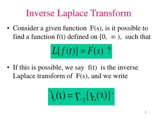
9. 4.2.2 Laplace Transform Representation. • H(s) is the Laplace Transform of h(t) and.. thus the h(t) is the inverse Laplace transform of H(s). • The Laplace transform of x(t) is • The Inverse Laplace Transform of X(s) is • We can express the relationship with the notation

10. 4.2.3 Convergence. • The condition for convergence of the Laplace transform is the absolute integrability of x(t)e-at , • The range of s for which the Laplace transform converges is termed the region of convergence (ROC) Figure 4.2: The Laplace transform applies to more general signals than the Fourier transform does. (a) Signal for which the Fourier transform does not exist. (b) Attenuating factor associated with Laplace transform. • (c) The modified signal x(t)e -tis absolutely integrable for  > 1.

11. 4.2.4 The s-Plane. • It is convenience to represent the complex frequency s graphically in terms of the s-plane. (i) the horizontal axis represents the real part of s (exponential damping factor s). (ii) The vertical axis represents the imaginary part of s (sinusoidal frequency w) • In s-plane, s =0 correspond to imaginary axis. • Fourier transfrom is given by the Laplace transform evaluated along the imaginary axis.

12. Cont’d… • The jw-axis divides the s-plane in half. (i) The region to the leftof the jw-axis is termed the left half of the s-plane.(ii) The region to the right of the jw-axis is termed the right half of the s-plane. • The real part of s is negative in the left half of the s-plane and positive in the right half of the s -plane.. Figure 4.3: The s-plane. The horizontal axis is Re{s}and the vertical axis is Im{s}. Zeros are depicted at s = –1 and s = –4  2j, and poles are depicted at s = –3, s = 2  3j, and s = 4.

13. 4.2.5 Poles and Zeros. • Zeros. The ck are the root of the numeratorpolynomial and are termed the zeros of X(s). Location of zeros are denoted as “o”. • Poles. The dk are the root of the denominator polynomial and are termed the poles of X(s). Location of poles are denoted as “x”. • The Laplace transform does not uniquely correspond to a signal x(t) if the ROC is not specified. • Two different signal may have identical Laplace Transform, but different ROC. Below is the example. Figure 4.4a Figure 4.4b Figure 4.4a. The ROC for x(t) = eatu(t) is depicted by the shaded region. A pole is located at s = a. Figure 4.4b. The ROC for y(t) = –eatu(–t) is depicted by the shaded region. A pole is located at s = a.

14. Example 4.1:Laplace Transform of a Causal Exponential Signal. Determine the Laplace transform of x(t)=eatu(t). Solution: Step 1: Find the Laplace transform. To evaluate e-(s-a)t, Substitute s=s + jw

15. Cont’d… Figure 4.5: The ROC for x(t) = eatu(t) is depicted by the shaded region. A pole is located at s = a. If s > 0, then e-(s-a)t goes to zero as t approach infinity, while as t is zero, e-(s-a)t goes to minus one, hence *The Laplace transform does not exist for s=<a because the integral does not converge. *The ROC is at s>a, the shaded region of the s-plane in figure below. The pole is at s=a. • .

16. 4.3 The Unilateral Laplace Transform and Properties. • The Unilateral Laplace Transform of a signal x(t) is defined by • The lower limit of implies that we do include discontinuities and impulses that occur at t = 0 in the integral. H(s) depends on x(t)for t >= 0. • The relationship between X(s) and x(t) as • The unilateral and bilateral Laplace transforms are equivalent for signals that are zero for time t<0.

17. Cont’d… Properties of Unilateral Laplace Transform. Scaling Linearity, For a>0 Time Shift for all t such that x(t - t)u(t) = x(t - t)u(t - t) • A shift in t in time correspond to multiplicationof the Laplace transform by the complex exponential e-st.

18. Cont’d… s-Domain Shift • Multiplication by a complex exponential in time introduces a shift in complex frequencys into the Laplace transform. Figure 4.6: Time shifts for which the unilateral Laplace transform time-shift property does not apply. (a) A nonzero portion of x(t) that occurs at times t 0 is shifted to times t < 0. (b) A nonzero portion x(t) that occurs at times t < 0 is shifted to times t  0.

19. Cont’d… Convolution. • Convolution in time domain corresponds to multiplication of Laplace transform. This property apply when x(t)=0 and y(t) = 0 for t < 0. Differentiation in the s-Domain. • Differentiation in the s-domain corresponds to multiplication by -t in the time domain.

20. Cont’d… Differentiation in the Time Domain. Initial and Final Value Theorem. • The initial value theorem allow us to determine the initial value, x(0-), and the final value, x(infinity), of x(t) directly from X(s). • The initial value theorem does NOT apply to rational functions X(s) in which the order of the numerator polynomial is greater than or equal to that of the denominator polynomial.

21. Example 4.2:Applying Properties. Find the unilateral Laplace Transform of x(t)=(-e3tu(t))*(tu(t)). Solution: Find the Unilateral Laplace Transform. And Apply s-domain differentiation property, Use the convolution property, • . 1

22. 4.4 Inversion of the Unilateral Laplace Transform. • We can determine the inverse Laplace transforms using one-to-one relationship between the signal and its unilateral Laplace transform. Appendix D1 consists of the table of Laplace Transform. • X(s) is the sum of simple terms, • Using the residue method, solve for a system linear equation. • Then sum the Inverse Laplace transform of each term.

23. Example 4.3:Inversion by Partial-Fraction Expansion. Find the Inverse Laplace Transform of Solution: Step 1: Use the partial fraction expansion of X(s) to write Solving the A, B and C by the method of residues

24. Cont’d…

25. Cont’d… A=1, B=-1 and C=2 Step 2:Construct the Inverse Laplace transform from the above partial-fraction term above. - The pole of the 1st term is at s = -1, so - The pole of the 2nd term is at s = -2, so -The double pole of the 3rd term is at s = -2, so Step 3: Combining the terms. • .

26. Example 4.4:Inversion An Improper Rational Laplace Transform. Find the Inverse Laplace Transform of Solution: Step 1: Use the long division to espress X(s) as sum of rational polynomial function. We can write,

27. Cont’d… Use partial fraction to expand the rational function, Step 2:Construct the Inverse Laplace transform from the above partial-fraction term above. Refer to the Laplace transform Table. • .

28. 4.5 Solving Differential Equation with Initial Condition. • Primary application of unilateral Laplace transform in system analysis, solving differential equations with nonzero initial condition. • Refer to the example.

29. Figure 4.7: RC circuit for Examples 6.4 and 6.10. Note that RC = 1/5. Example 4.5:RC Circuit Analysis (Initial condition) Use the Laplace transform to find the voltage across the capacitor , y(t), for the RC circuit shown in Figure 4.7 in response to the applied voltage x(t)=(3/5)e-2tu(t) and the initial condition y(0-) = -2. Solution: Step 1: Derive differential equation from the circuit. KVL around the loop.

30. Cont’d… Step 2: Get the unilateral Laplace Transform. Apply the properties of differential in time domain, Step 3: Substitute Unilateral Laplace Transform of x(t) into Y(s). Laplace transform of the applied voltage, x(t); Given initial condition, substitute y(0-)=-2 into (2), And substitute (3) into (2),

31. Cont’d… Step 4: Expand Y(s) into partial fraction. Step 5: Take Inverse Unilateral Laplace Transform of Y(s). by referring to the Laplace transform table. • .

32. QUIZ 1 Use the basic Laplace transforms & Laplace transform properties in Appendix D to determine the following signals: a) b) c)

33. QUIZ 2 • Use the method of partial fractions to find the time signals corresponding to the following Laplace transforms: • a) • b) • C)

34. 4.6 Forced and Natural Responses in Unilateral Laplace Transform. • Primary application of the unilateral Laplace transform is to solve differential equations with non-zero initial conditions. • The initial conditions are incorporated into the solution as the values of the signal and its derivatives that occur at time zero in the differentiation property. • General form of differentiation property:-

35. 4.6 Forced and Natural Responses in Unilateral Laplace Transform. • The forced response of a system represents the component of the response associated entirely with the input, denoted as . This response represents the output when the initial conditions are zero. • The natural response represents the component of the output due entirely to the initial conditions, denoted as . This response represents the system output when the input is zero.

36. Example 4.6: Finding forced and natural responses. Use the unilateral Laplace transform to determine the output of a system represented by the differential equation, in response to the input . Assume that the initial conditions on the system are; Solution. Using differentiation property in Eq. 6.19 and taking Laplace transform of both sides of the differential equation,

37. Contd… Rearranging the terms; Solving for Y(s), we get; The first term is associated with the forced response , . The second term corresponds to the natural response, . Using the transform of input, and the initial conditions, we obtain; and

38. Contd… Next, taking the inverse Laplace transforms of and , we obtain; and Hence, the output of the system is;

39. Contd… • a) Forced response of the system, y(f)(t). (b) Natural response of the system, y(n)(t). (c) System output.

40. 4.7 Properties of Bilateral Laplace Transform. • The Bilateral Laplace Transform is suitable to the problems involving non-causal signals and system. • The properties of linearity, scaling, s-domain shift, convolution and differentiation in the s-domain is identicalfor the bilateral and unilateral LT, the operations associated by these properties may change the ROC. • Example; a linearity property. • ROC of the sum of the signals is an intersection of the individual ROCs.

41. Cont’d… Time Shift • The bilateral Laplace Transform is evaluated over both positive and negative values of time. ROC is unchanged by a time shift. Differentiation in the Time Domain. • Differentiation in time domain corresponds to multiplication by s.

42. Cont’d… Integration with Respect to Time. • Integration corresponds to division by s • Pole is at s=0, we are integrating to the right, hence the ROC must lies to the right of s=0.

43. 4.8 Inversion of Bilateral Laplace Transform. • The inversion of Bilateral Laplace transforms are expressed as a ratio of polynomial in s. • Compare to the unilateral, in the bilateral Laplace transform we must use the ROC to determine the unique inverse transform in bilateral case.

44. Example 4.7:Inverting a Proper Rational Laplace Transform. Find the Inverse bilateral Laplace Transform of With ROC -1<Re(s)<1. Solution: Step 1: Use the partial fraction expansion of X(s) to write Solving the A, B and C by the method of residues

45. Cont’d… Step 2:Construct the Inverse Laplace transform from the above partial-fraction term above. - The pole of the 1st term is at s = -1, the ROC lies to the right of this pole, choose the right-sided inverse Laplace Transform. - The pole of the 2nd term is at s = 1, the ROC is to the left of the pole, choose the left-sided inverse Laplace Transform. -The pole of the 3rd term is at s = -2, the ROC is to the right of the pole, choose the right-sided inverse Laplace Transform.

46. Cont’d… Step 3: Combining the terms. • Combining this three terms we obtain, Figure 4.12 : Poles and ROC for Example 6.17.

47. 4.9 Transfer Function. • The transfer function of an LTI system is defined as the Laplace transform of the impulse response. • Take the bilateral Laplace transform of both sides of the equation and use the convolution properties, it results in; • Rearrange the above equation will result in the ratio of Laplace transform of the output signal to the Laplace transform of the input signal. (Note: X(s) is non-zero)

48. 4.9.1 Transfer Function and Differential-Equation System Description. Given a differential equation. Step 1: Substitute y(t) = estH(s) into the equation. y(t) = estH(s), substitute to the above equation result in, Step 2: Solve for H(s). H(s) is a ratio of polynomial and s is termed as rational transfer function.

49. Example 4.8:Find the Transfer Function. Find the transfer function of the LTI system described by the differential equation below, Solution: Step 1:estis an eigenfunction of LTI system. If input, x(t)=est Then, y(t) = estH(s). Hence, substitute into the equation.. Step 2: Solve for H(s).

50. Cont’d… Hence, the transfer function is, • .