biogenic, pryogenic, anthropogenic
230 likes | 459 Vues
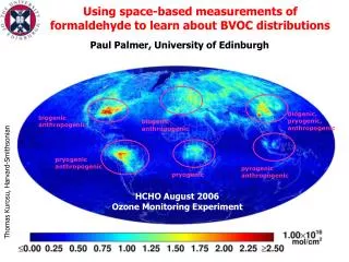
biogenic, pryogenic, anthropogenic. biogenic anthropogenic. biogenic anthropogenic. pryogenic anthropogenic. pyrogenic anthropogenic. pryogenic. Using space-based measurements of formaldehyde to learn about BVOC distributions. Paul Palmer, University of Edinburgh.

biogenic, pryogenic, anthropogenic
E N D
Presentation Transcript
biogenic, pryogenic, anthropogenic biogenic anthropogenic biogenic anthropogenic pryogenic anthropogenic pyrogenic anthropogenic pryogenic Using space-based measurements of formaldehyde to learn about BVOC distributions Paul Palmer, University of Edinburgh Thomas Kurosu, Harvard-Smithsonian HCHO August 2006 Ozone Monitoring Experiment
hv O3 NO2 NO OH HO2 HC+OH HCHO + products Tropospheric O3 is an important climate forcing agent NOx, HC, CO Level of Scientific Understanding Natural VOC emissions (50% isoprene) ~ CH4 emissions. IPCC, 2001
MEGAN Isoprene Emission Inventory • Environmental factors: • temperature • solar irradiance • leaf area index • leaf age July 2003
Global Ozone Monitoring Experiment (GOME) &the Ozone Monitoring Instrument (OMI) GOME Launched in 2004 • GOME (European), OMI (Finnish/USA) are nadir SBUV instruments • Ground pixel (nadir): 320 x 40 km2 (GOME), 13 x 24 km2 (OMI) • 10.30 desc (GOME), 13.45 asc (OMI) cross-equator time • GOME: 3 viewing angles global coverage within 3 days • OMI: 60 across-track pixels daily global coverage • O3, NO2, BrO, OClO, SO2, HCHO, H2O, cloud properties
HCHO Column Abundance Fitted in a Narrow UV Spectral Window 226-356 nm fitting window Fitting uncertainty of slant columns is typically < 4x10¹⁵ molec cm-2
vertical column = slant column /AMF GEOS-CHEM satellite lnIB/ Sigma coordinate () dHCHO 1 Earth Surface HCHO mixing ratio C() Scattering weights Shape factor S() = C() air/HCHO w() = - 1/AMFGlnIB/ 1 AMF = AMFG w() S() d 0
0.5 2 2.5 1 0 1.5 [1016 molec cm-2] GOME HCHO columns – fractionally cloudy pixels (>40%) removed Biogenic emissions Biomass burning July 2001 Data: c/o Chance et al * Columns fitted: 337-356nm * Fitting uncertainty < continental signals
hours hours HCHO h, OH OH kHCHO ___________ HCHO EVOC = (kVOCYVOCHCHO) WHCHO Isoprene a-pinene propane 100 km Distance downwind VOC source Relating HCHO Columns to VOC Emissions VOC Net Local linear relationship between HCHO and E EVOC: HCHOfromGEOS-CHEM CTM and MEGAN isoprene emission model Palmer et al, JGR, 2003.
Modeling Overview MCM: parameterized HCHO source from monoterpenes and MBO GEOS-CHEM global 3D chemistry transport model PAR, T Emissions MODEL BIOSPHERE MEGAN (isoprene) Canopy model Leaf age LAI Temperature Fixed Base factors GEIA Monoterpenes MBO Acetone Methanol Monthly mean AVHRR LAI
NOx = 1 ppb NOx = 0.1 ppb MCM HCHO yield calculations 0.5 Isoprene C5H8+OH(i) RO2+NOHCHO, MVK, MACR (ii) RO2+HO2ROOH ROOH recycle RO and RO2 Cumulative HCHO yield [per C] Higher CH3COCH3 yield from monoterpene oxidation delayed (and smeared) HCHO production HOURS 0.4 Parameterization (1ST-order decay) of HCHO production from monoterpenes in global 3-D CTM pinene ( pinene similar) DAYS Palmer et al, JGR, 2006.
Seasonal Variation of Y2001 Isoprene Emissions May Aug Jun Sep 1012 atom C cm-2s-1 Jul 7 0 3.5 MEGAN GOME MEGAN GOME • Good accord for seasonal variation, regional distribution of emissions (differences in hot spot locations – implications for O3 prod/loss). • Other biogenic VOCs play a small role in GOME interpretation Palmer et al, JGR, 2006.
MEGAN Obs GOME Isoprene flux [1012 C cm-2 s-1] Julian Day, 2001 Sparse ground-truthing of GOME HCHO columns and derived isoprene flux estimates Seasonal Variation: Comparison with eddy correlation isoprene flux measurements (B. Lamb) is encouraging May Jun July Aug Sep Atlanta, GA 199619971998199920002001 PROPHET Forest Site, MI Atlanta, GA GOME HCHO [1016 molec cm-2] Interannual Variation: Correlate with EPA isoprene surface concentration data. Outliers due to local emissions. PAMS Isoprene, 10-12LT [ppbC]
May Jun Jul Aug Sep 1996 1997 1998 1999 2000 2001 GOME Isoprene Emissions: 1996-2001 Palmer et al, JGR, 2006. [1012 molecules cm-2s-1] 10 0 5
Surface temperature explains 80% of GOME-observed variation in HCHO G98 fitted to GOME data GOME Isoprene Emissions [1012 atoms C cm-2s-1] G98 Modeled curves NCEP Surface Temperature [K] Palmer et al, JGR, 2006. Time to revise model parameterizations of isoprene emissions?
Tropical ecosystems represent 75% of biogenic NMVOC emissions What drives observed variability of tropical BVOC emissions?
Significant pyrogenic HCHO source over tropics Good: Additional trace gas measurement of biomass burning; effect can be identified largely by firecounts (see below) Bad: Observed HCHO a mixture of biogenic and pyrogenic – difficult to separate without better temporal and spatial resolution GOME Sep 1997 1997 1998 1999 2000 2001 X = Active Fire (ATSR) Monthly ATSR Firecounts Slant Column HCHO [1016 molec cm-2] Nov 1997 Day of Year
In situ isoprene 2002 HCHO and Isoprene over the Amazon Trostdorf et al, 2004 GOME 1997 1998 1999 2000 2001 ATSR Firecounts used to remove HCHO from fires
Isoprene Limonene [ppb] monoterpene emission of Apeiba tibourbou 1500 40 1000 30 [°C] (µmol m-2 s-1) PAR 500 20 Beta-pinene temperature 10 6 limonene myrcene 5 b-pinene a-pinene 4 sabinene 3 (µg g-1 h-1) G93 for isop. emission rate (C) [sum of monoterpenes] 2 1 0 4 4 2 2 (mmol m-2 s-1) transpiration Time of Day (mg g-1 h -1) assimilation (C) 0 0 12:00 00:00 00:00 12:00 00:00 06:00 18:00 06:00 18:00 local time [hh:mm] Can isoprene explain the observed magnitude and variance of HCHO columns over the tropics? Africa Amazon C/o J. Kesselmeier C/o J. Saxton A. Lewis
May Jul Jun Sep Oct Aug OMI gives a better chance of estimating African BVOCs OMI Data c/o Thomas Kurosu; horizontal resolution O(10x25 km2)
[ppt] Isoprene concentrations during AMMA July 2006 measured by the Bae146 aircraft; MODIS tree cover overlaid OMI ATSR Firecounts Jul Jul Isoprene data c/o Jim Hopkins and Ally Lewis, U. York
O3 > 100 ppb on 6 consecutive days Estimated up to 700 extra deaths attributable to air pollution (O3 and PM10) in UK during this period 2pm, 6th Aug, 2003 “Normal” airmass flow 1400 40 35 1200 Isoprene (ppt) 30 Temperature (C) 1000 25 800 20 600 15 Stagnant airmass flow 400 10 200 5 0 0 4-Aug 2-Aug 6-Aug 8-Aug 27-Jul 29-Jul 31-Jul 12-Aug 16-Aug 10-Aug 14-Aug 18-Aug 20-Aug 22-Aug 24-Aug 26-Aug 28-Aug 30-Aug Compiled from UK ozone network data An increasing role for BVOCs in UK air quality? Isoprene c/o Ally Lewis
Monoterpenes BVOC fluxes for a “hot, sunny” day Isoprene Stewart et al, 2003 The European Heatwave of 2006 Jul Aug Jun Satellite observations test bottom-up emission inventories used for air quality: an important step toward regional chemical weather forecasting
Final Comments Proper interpretation of HCHO requires an integrated approach, i.e., including surface data, lab data Interpreting space-based HCHO data is still in its infancy – new instruments bring better resolution but also new challenges With the frequency of European heatwaves projected to increase the role of BVOCs in future UK air quality must be better quantified