Download

1 / 31
320 likes | 496 Vues
Optimal Eye Movement Strategies In Visual Search. Visual Accuity. http://www.svi.cps.utexas.edu/HamiltonCreek.mov. Images from Laura Walker Renninger. http://www.svi.cps.utexas.edu/foveator.htm. Attention (And Fixation) Shifting Strategies. Visual Saliency

E N D
Visual Accuity • http://www.svi.cps.utexas.edu/HamiltonCreek.mov
Attention (And Fixation) Shifting Strategies • Visual Saliency • Attend to what stands out from background • Experience Guided Search (last class) • Attend to locations of maximum posterior probability (MAP) • Information Maximization • Given low resolution in parafovea, perhaps we move our eyes to gather as much information as possible. • Low resolution in parafovea -> uncertainty • Move eyes to reduce this uncertainty (= gather information) • Information maximization and MAP both predict task specificity of eye movements.
Najemnik & Geisler (2005) • 1/f noise • same statistics as natural images • Target • sine wave grating • Manipulations • Target contrast • Background noise contrast
Measuring Visibility At Fovea • Subject fixates at center • Two displays in quick succession • Task: determine which one contains the target grating • Measure accuracy as a function of target and background contrast at each location • For center location: • Threshold = 82% accuracy
Derive Discriminability Curves • For a given background contrast and target contrast • d’: signal to noiseratio • If noise is Gaussian,1/d’2 is variance ofnoisedistribution • Two noise components • external noise: dueto 1/f background • internal noise: due toinefficiency of sensory system background contrast .05, target contrast .07 background contrast .20 and target contrast .19
Terminology d’E(i): discriminability due to external noise at location i d’I(i,k(t)): discriminability at location i due to internal noise given fixation at current time is k(t) Combined noise from two independent Gaussian sources:
Snapshot Likelihood (Observation) Model • Imagine a feature detector at each location that matches the target template (grating) against the visual information at that location • Wi,k(t): Observation at location i at time t when fixation at k(t) • Mean = 0.5 if target present, -0.5 if target absent • Drawn from Gaussian with variance g[i,k(t)]-1
Integrating Sequence Of Observations • Sequence of t=1…T fixations • At each fixation, obtain noisy evidence concerning target presence at each location i • Wk(1),Wk(2), … Wk(T) • Bayesian ideal observer:
Quiz • Are the W’s independent conditioned on a location(i or j)? • It depends on nature of internal and external noise.
Conditioning On External Noise • xi: (unknown) external noise at location I • Marginalize out over x: • Assuming internal noise is independent over time and space of external noise: • And external noise is independent over space:
Conjugate Priors To The Rescue • Because internal noise and external noise are Gaussian, • Integral can be computed analytically. • Gaussian prior • Gaussian likelihood • -> Gaussian posterior = +1 if q=i, -1 otherwise
Conjugate Priors To The Rescue • Form of likelihood: • Form of posterior: • But ugly constant is the same in numerator and denom.
Final Result With • Intuitive result Weighted sum of evidence, where weight ~ reliability Simple incremental rule for computing over time Related to 1/variance Of observation
What We Haven’t Discussed Yet • How is next fixation location chosen? • Go to location most likely to contain target (MAP location) • Go to location that will obtain the greatest expected reduction in uncertainty (entropy) • Go to location that will obtain information that will maximize probability of correctly identifying target • Comparison to random searcher • Ideal decision maker, but chooses fixations randomly
Choosing Next Fixation: Some Ugly Details C: correct identification of target Depends on meanand variance ofprobability densityfor an observation Normal density Normal cdf
Average Spatial Distribution Of FixationsFor 1st, 3d, and 5th SaccadesIdeal and Human Observers
Results I • Median # fixations to locate target, as a function of foveated target’s visibility • Background noise contrast = .025 solid = ideal searcher • Background noise contrast = .20 dashed = random searcher Observer 1 Observer 2
Results II • Median number of fixations to locate target as a function of target eccentricity (x axis) and target visibility in fovea (d’) • Background noise contrast = .05Background noisecontrast = .20 • Solid = ideal observer • Dots = medians(less reliable atsmall eccentricities)
Results III • Posterior probability at target location as a function of the number of fixations prior to finding target • dashed = random searcher • solid = ideal observer
Are Fixations Information Seeking? • Comparison to MAP selection • Can’t distinguish
Distribution of Fixations • MAP selection vs. information seeking
Distribution of Fixations II • Direction of fixations relative to center of display • Confirms previous result
Take Home • Visual search can be cast as optimal • Optimal choice of next fixation • Possibly not optimal integration of information over fixations • …subject to limitation on quality of visual information • Noise in images • Acuity limitation of retina
Take Home II • We’ve discussed several Bayesian accounts that cast vision and attention in terms of ideal observers. • How does this analysis give us insight into how the visual system works? • Rigorous starting point for developing models • Provides well motivated computational framework • Can ask how human behavior deviates from optimal computation • Can ask how people achieve near-optimal performance with imperfect, noisy neural hardware