COMP4048 3D Visualisation, Interaction and Navigation
COMP4048 3D Visualisation, Interaction and Navigation. Richard Webber National ICT Australia. Lecture Overview. 3D – What, How and Why 3D Graph Drawing 2D 3D Genus > 0 The extra dimension Viewpoint selection. 3D Computer Graphics. (Foley et al. 1990, Szirmay-Kalos et al. 1995)

COMP4048 3D Visualisation, Interaction and Navigation
E N D
Presentation Transcript
COMP40483D Visualisation, Interaction and Navigation Richard WebberNational ICT Australia
Lecture Overview • 3D – What, How and Why • 3D Graph Drawing • 2D 3D • Genus > 0 • The extra dimension • Viewpoint selection
3D Computer Graphics • (Foley et al. 1990, Szirmay-Kalos et al. 1995) • Vertices have 3 coordinate – x, y, z • Edges are routes through 3d points • 3d model 2d image = projection • Orthographic parallel– architectural plans • Perspective– 3d computer games • Fisheye-lens– context+focus
3D Computer Graphics • Orthographic Parallel Projection • Less realistic, but simplifies the math
3D Computer Graphics • Perspective Projection • Standard in modern hardware
3D Computer Graphics • Fisheye-lens Projection • Provides focus+context
The Illusion of 3D • The Necker Cube Illusion (Foley et al. 1990) • Is the wireframe cube facing down and left or up and right? = or
The Illusion of 3D • Adding extra information removes ambiguities • Depth cueing (fog)
The Illusion of 3D • Shadows (projections)
The Illusion of 3D • Perspective cues (Ware 2000)
The Illusion of 3D • Perspective cues (Ware 2000)
The Illusion of 3D • Stereoscopic Displays • Stereo image pairs • Stereoscopic Displays • Random-dot stereograms
The Illusion of 3D • Stereoscopic Displays • Head-mounted displays (immersive VR)
The Illusion of 3D • Stereoscopic Displays • “Filtering” glasses (fishtank VR)
The Illusion of 3D • Kinetic Depth Effect (Wallach, O’Connell 1953) • Produces the illusion of 3d in a 2d projection by rotating/rocking the graph • Direction of rotation can be ambiguous
Why 3D? (Ware, Franck 1996) • Intuition • More natural – we live in a 3d world • Greater “volume” for information
Why 3D? • Anecdotal evidence (applications) • SemNet (Fairchild et al. 1988) • Lyberworld (Hemmje et al. 1994) • Information Visualizer (Mackinlay 1992)
Why 3D? • Sollenberger and Milgram 1993 • Finding paths in a 3d graph drawing • stereoscopic glasses > static projection • continuous rotation > static projection • unidirectional user rotation = continuous rotation • rotation + stereoscopic >> static projection
Why 3D? • Ware and Franck 1996 • bidirectional user rotation > unidirectional user rotation • head-controlled parallax = bidirectional user rotation “the size of graph that can be traced with the same accuracy increases three-fold with the use of stereoscopic display and rotation”
3D by Physical Analogy • Springs adapt very easily • E.g., Bruß and Frick 1995 • Distance and direction work in any dimension • Other energy-based systems also adapt • Equations can get harder • Simulated annealing can do anything • The state space may get larger
3D DAG Drawings • Place layers in parallel planes • Barycentering now in 2d • What is an edge “crossing”? • Restrict to surface of genus 0 solids • Edge crossing problem circular • Both of these approaches are sometimes referred to as 2½d
Genus > 0 Surfaces (Garvan 1997) • Genus = “number of holes/handles” • Genus 0: plane, sphere, cylinder, cone, cube • Genus 1: torus (doughnut), teacup • Genus 2: two-handed teacup • Genus 3: ABC logo, pretzel • Genus g: Swiss cheese • Genus g graph can be drawn on a genus g surface without edge crossings
The Extra Dimension • Draw a 2d graph then use 3rd (and more) dimensions for extra information • Dimensions = x, y, z, size, shape, colour, … • Draw multiple 2d graphs (abstractions) using the 3rd dimension • Cluster graphs (Feng 1997) • Look “through” to lower layers
3d Input Techniques • Using a traditional (WIMP) interface places stress on the user
3d Input Techniques • 3D-specific input devices • Spaceball/Spacemouse • “Flying” mice
3d Input Techniques • 3D-specific input devices • Dataglove
3d Input Techniques • First-person-shooter computer games provide a good grounding in using traditional devices for 3d navigation
Viewpoint Selection • Wouldn’t it be nice if you could tell the computer • roughly where you want to be • what you want to look at and the computer responded by moving you smoothly to a suitable position and orientation? • Where and what could be spatial or semantic
Viewpoint Selection • Avoiding viewpoints that are “bad” • Aspect Graphs (Plantinga, Dyer 1990) • Bad = can’t see many faces of a 3d solid • Kamada and Kawai 1988 • Bad = non-general “shape” information of the drawing is lost
Viewpoint Selection • Bose et al. 1995 • Bad = degenerate with respect to some computational geometry problem • Regular and Wirtinger projections • Webber 1998 • Bad = “the apparent abstract graph of the 2d drawing differs from the abstract graph of the 3d model” there is an occlusion
Viewpoints and Occlusions • Vertex-Vertex Occlusions • Also vertex-edge, edge-vertex and (coplanar) edge-edge occlusions
Viewpoints and Occlusions • Can characterise all bad viewpoints • Note symmetry: (a, b) = (b, a)
Viewpoints and Occlusions • Can check a single viewpoint in O(|V0|2+|V||E|) time • Can preprocess to check many viewpoints against the same drawing • O(|S| log |S|) preprocessing time • |S| is O(|V0|2+|V||E|+kbva); kbva is O(|V0|2+|V|2|E|2) • Check viewpoints in logarithmic time
Best Viewpoints • Finding viewpoints that are “best” • Kamada and Kawai 1988 • Most general viewpoints • Bose et al. 1995 • Viewpoints with least edge crossings • Their models can yield best viewpoints using our techniques
Best Viewpoints • Goodness of a viewpoint = how far it is from the nearest bad viewpoint (Webber 1998) • Rotational Separation Diagram (RSD) • Goodness = great-circle distance • O(|S| log |S|) preprocessing time • Good for interacting with drawings • Observed Separation Diagram (OSD) • Goodness = apparent distance between elements in 2d image • Good for static presentation (journals)