Chapter 5 Finance Application

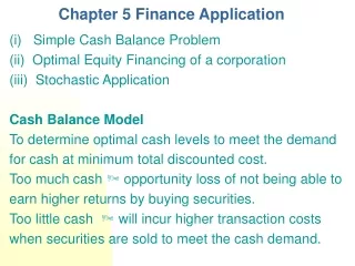
1. Chapter 5 Finance Application (i) Simple Cash Balance Problem (ii) Optimal Equity Financing of a corporation (iii) Stochastic Application Cash Balance Model To determine optimal cash levels to meet the demand for cash at minimum total discounted cost. Too much cash  opportunity loss of not being able to earn higher returns by buying securities. Too little cash  will incur higher transaction costs when securities are sold to meet the cash demand.

2. NOTATION T = the time horizon, x(t) = the cash balance in $. y(t) = the security balance in $. d(t) = instantaneous cash demand (d(t)<0  accounts receivable.) u(t) = sale of securities, -U2 u  U1 (u<0  purchase), U2 0,U1 0. r1(t) = interest on Cash (demand deposits). r2(t) = interest on Securities (e.g. bonds).  = Broker’s Commission in dollars per dollar’s worth of Securities bought or sold.

3. State Equations Control constraints Objective Solution. By Maximum Principle

4. Interpretation:1(t) is the future value (at timeT ) of one dollar held in the cash account from time t to T. 2(t) is the future value (at timeT ) of one dollar in invested securities from time t to T. Thus, the adjoint variables have natural interpretations as the actuarial evaluations of competitive investments at each point of time.

5. Optimal Policy In order to deal with the absolute value function we write the control variables u as the difference of two nonnegative variables,i.e., we impose the quadratic constraint Given (5.10) and (5.11) we can write

6. We can now substitute (5.10) and (5.12) into the Hamiltonian (5.5) and reproduce below the part which depends on control variables u1 and u2 , and denote it by W. Thus, W is linear in u1 and u2 so that the optimal strategy is bang-bang and is as follows: where

7. Interpretation: Sell at the max allowable rate if the future value of a dollar less than broker’s commission (i.e. the future value of (1-) dollars ) is greater than the future value of a dollar’s worth of securities, and not to sell if the future values are in reverse order. Interpretation:  u2* =U2 i.e.,purchase securities at the maximum rate if the future value of a dollar plus broker’s commission is less than the future value of a dollar’s worth of securities.

8. Figure 5.1: Optimal Policy Shown in ( 1,2) Space

9. Figure 5.2: Optimal Policy Shown in ( t,2/1) Space

10. Optimal Financing Model y(t) = the value of the firm’s assets or invested capital at time t, x(t) = the current earnings rate in dollars per unit time at time t, u(t) = the external or new equity financing expressed as a multiple of current earnings; u0, (t) = the fraction of current earnings retained,i.e.,1- (t) represents the rate of dividend payout; 0(t) 1, 1-c = the proportional floatation (i.e.,transaction) cost for external equity; c a constant, 0 c 1,  = the continuous discount rate (assumed constant); known commonly as the stockholder’s required rate of return, r = the actual rate of return (assumed constant) on the firm’s invested capital; r > , g = the upper bound on the growth rate of the firm’s assets, T = the planning horizon; T< ( T=  in section 5.2.4)

11. Objective: Maximize the net present value of future dividends that accrue to the initial shares.That is, Assume no salvage value for the time being. For convenience, we restate this problem as

12. Solution. By Maximum Principle the current-value Hamiltonian the current-value adjoint variable  satisfies with the transversality condition Rewrite the Hamiltonian as where

13. So given , u* is defined by max ( W1u+W2 ), subject to u0, 0 1, cu+  g/r, which is an LP. This is a generalized bang-bang (i.e,extreme point) solution. The Hamiltonian maximization problem can be stated as follows: we have two cases: Case A:g r and Case B:g > r , under each of which,we can solve the linear programming (5.40) graphically in a closed form. This is done in Figure 5.4 and Figure 5.5.

14. Figure 5.4 Case A: g  r

15. Figure 5.5 Case B: g > r

16. Table 5.1 Characterization of Optimal Controls

17. Synthesis of Optimal Paths Define the reverse-time variable as so that The transversality condition on the adjoint variable Let Using the definitions of and and the conditions (5.42) and (5.41), we can write reverse-time versions of (5.30) and (5.35) as follows:

18. Case A: g  r Feasible subcases are A1, A3, and A6. (0)=0  W1(0)=W2(0)=-1  A1 Subcase A1: we have Since 0 c <1,  Thus, to stay in this subcase requires that must remain negative for some time as increases.  is increasing asymptotically toward the value 1/ W2 is increasing asymptotically toward the value r/ - 1

19. Since r >  , there exists , such that So, the firm exits subcase A1 provided Remarks: i) We assume T sufficiently large so that the firm will exit A1 at . ii) Note that for r < , the firm never exits from Subcase A1. Obviously, no use investing if the rate of return is less than the discount rate. iii) At , W2 =0, W1<0  Subcase A6.

20. Subcase A6: The optimal controls The optimal controls are obtained by conditions required to sustain W2=0 for a finite time interval. substitute =1/r (since W2=0), and equating the right-hand to zero we obtain We have assumed r>,so we cannot maintain singular control. Since r > , Therefore, W2is increasing from zero and becomes positive after . Thus, at , we switch to subcase A3.

21. Subcase A3: The optimal controls: The state and the adjoint equations are: Since ,  is increasing at from its value of 1/r. (i) >g : As increases, decreases and becomes zero at a value obtained by equating the right-hand side of (5.53) to zero,i.e., at

22. Since r >  > g , The firm will continue to stay in A3. (ii)   g: As increases, increases. So . The firm continues to stay in Subcase A3.

23. Figure 5.6: Optimal Path for Case A: gr

24. Interpretation: Control switches to u*=*=0 at . i.e, it requires at least units of time to retain a dollar of earnings to be worthwhile. That means, it pays to invest as much earnings as feasible before and it does not pay to invest any earnings after .Thus, is the point of indifference between retaining earnings or paying dividends out of earnings. Suppose the firm invests one dollar of earnings at . Since this is the last time any earnings invested will pay off, it is obvious that this dollar will yield dividends at the rate r from to T. (i.e, under the optimal policy)

25. The value of this dividend stream in terms of dollars is But this must be equated to one dollar to find the indifference point,i.e., So under the optimal policy: The firm grows at rate g until ,Since g  r, the entire growth can be financed out of retained earnings. Thus, there is no need to resort to external financing which is more expensive (0 c 1). Then from , the firm issues dividends since there is no salvage value at T.

26. Case B: g > r Since g/r >1, the constraint   1 is relevant. Subcase B1: The analysis is the same as subcase A1. The firm swithches out at time to subcase B8. Subcase B8: The optimal controls are: As in subcase A6, the singular case cannot be sustained since r >  . W2 is increasing at from zero and becomes positive after .Thus, at ,the firm find itself in subcase B4.

27. Subcase B4: The optimal controls are: The state and the adjoint equations are: Since ,we have As increases, W1increases and become zero at time defined by which gives At , the firms switches to subcase B7.

28. Subcase B7: The optimal controls are; To maintain this singularcontrol over a finite time period, we must keep W1= 0 in the interval. This means we must have which implies To compute , we substitute (5.64) into (5.44) and obtain: Substituting from (5.62) and equating the right-hand side to zero, we obtain Since r >  , the firm cannot stay in B7.

29. From (5.65), we have which implies that  is increasing and therefore, W1 is increasing.Thus at ,the firm switches to subcase B3. Subcase B3: The optimal controls are The reverse-time state and the adjoint equations are: Since , is increasing. In case B, we assume g > r, But r >  has been assumed throughout the

30. chapter. Therefore,  < g and the second term in the right-hand side of (5.69) is increasing. That means and continues to increase. Therefore, the firm continues to stay in subcase B3. Interpretation of Since external equity is more expensive than retained earnings as a source of financing, investment financed by external equity requires more time to be worthwhile. Thus, should be the time required to compensate for the floatation cost of external equity.

32. Figure 5.7: Optimal Path for Case B: g > r

33. 5.2.4 Solution for the Infinite Horizon Problem For the infinite horizon case the transversality condition must be changed to This condition is only a sufficient condition (not a necessary one). Case A: g  r The limiting solution in this case is given as subcase A3, i.e., and

34. For  > g, the analysis of subcase A3 shows that is increasing asymptotically toward the value Thus clearly satisfies (5.75). Furthermore, which implies that the firm stays in subcase A3, i.e, the maximum principle holds. Thus, The corresponding state trajectory . The adjoint trajectory

35. (5.76) reminds us of the Gordon’s classic formula. represents the marginal worth per additional unit of earnings. Obviously, a unit increase in earnings will mean an increase of 1- * or 1-g/r units in dividends. This should be capitalized at the rate equal to the discount rate less the growth rate (i.e.,  - g ). For   g, the reverse-time construction implies that increase without bound as increase. Thus, we do not have any  which satisfies the limiting condition in (5.75). Note that for   g, and infinite horizon, the objective function can be made infinite.

36. For example, any control policy with earnings growing at rate q[, g] coupled with a partial dividend payout (i.e., 0  1) has an infinite value for the objective function. That is, with , we have Case B:g > r The limit of the finite horizon optimal solution is to grow at the maximum growth rate with Since disappears in the limit, the stockholders will never collect dividends. The firm has become an infinite sink for investment.

37. Remarks: Let denote the optimal control for the finite horizon problem in Case B. Let denote any optimal control for the infinite horizon problem in Case B. We already know that . Define an infinite horizon control by extending as follows: We now note that for our model in Case B, we have Obviously, is not an optimal control for the infinite horizon problem.

38. If we introduce a salvage value Bx(T), B > 0, for the finite horizon problem, the new objective function, is a closed mapping in the sense that for the modified model.

39. Example 5.2: Solution: Since g  r  Case A , The optimal controls are The optimal state trajectory is;

40. The value of the objective function is; Infinite horizon solution Since g <  , and g < r, the problem is not ill-posed. The optimal controls are: and