Download
1 / 40
400 likes | 602 Vues
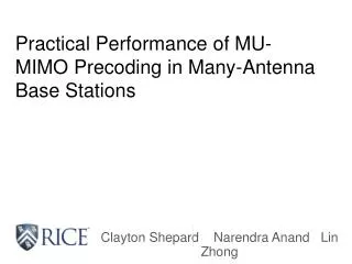
Practical Performance of MU-MIMO Precoding in Many-Antenna Base Stations. Clayton Shepard Narendra Anand Lin Zhong. Background: Many-Antennas. More antennas = more c apacity Traditional approaches don’t scale. Background: Beamforming. Destructive Interference. =.

E N D
Practical Performance of MU-MIMO Precoding in Many-Antenna Base Stations Clayton Shepard NarendraAnand Lin Zhong
Background: Many-Antennas • More antennas = more capacity • Traditional approaches don’t scale
Background: Beamforming Destructive Interference = Constructive Interference ? = 3
Background: Channel Estimation Due to environment and terminal mobility estimation has to occur quickly and periodically Path Effects (Walls) Align the phases at the receiver to ensure constructive interference BS + = +
Background: Channel Estimation BS Multiple users have to send pilots orthogonally
Frame Structure • Time Division Duplex (TDD) • Uplink and Downlink use the same channel estimates (Still Retrospective) Retrospectively Apply Coherence Time Channel Estimation Uplink … CE Comp Downlink Uplink CE … Pipeline Uplink Computational Overhead
Background: Zero-forcing Null Null Null Null Null Data 1
Background: Zero-forcing Data 2 Null Null Null Null Null
Background: Zero-forcing Data 2 Data 3 Data 1 Data 4 Data 5 Data 6
Background: Scaling Up Conjugate Data 2 Data 3 Data 1 Data 4 Data 5 Data 6
Conjugate vs. Zero-forcing • Negligible Processing • Completely Distributed • No Latency Overhead • Poor Spectral Efficiency • O(M•K2) • Centralized • Substantial Overhead • Good Spectral Efficiency
Under what scenarios, if any, does conjugate precoding outperform zero-forcing?
Performance Factors • Environmental • Complex, and constantly changing • Design • Straightforward and Static
Performance Factors • Environmental • Channel Coherence • Precoder Spectral Efficiency • Design • Number of Antennas • Hardware Capability
Environmental Factor: Channel Coherence • Coherence Time • Increases frequency of channel estimation • Coherence Bandwidth • Increases coherence bandwidth
Env. Factor: Precoder Spectral Efficiency • Real-world performance, neglecting overhead • Performance Depends on: • User Orthogonality • Propagation Effects • Noise • Interference • Can be modeled, but impossible to capture everything
Design Factor: Number of Antennas • Number of Base Station Antennas (M) • Increases amount of computation • Number of User Antennas (K) • Increases channel estimation and computation
Design Factor: Hardware Capability • Conjugate has negligible computational cost • Zero-forcing requires: • Bi-Directional Data Transport • Large Matrix Inversions
Zero-forcing Hardware Factors • Channel Bandwidth • Quantization • Inversion Latency • Data Transport • Switching Latency • Throughput
Without Considering Computation CE Comp Transmit
Spectral Efficiency vs. # of BS antennas K = 15 Spectral Efficiency (bps/Hz) # of Base Station Antennas (M)
Spectral Efficiency vs. # of Users M = 64 Spectral Efficiency (bps/Hz) # of Users (K)
Considering Computation CE Comp Transmit
M = 64 K = 15 Achieved Capacity (bps/Hz) Coherence Time (s) Zeroforcing with various hardware configurations
Performance vs. # of Users M = 64 Ct= 30 ms Achieved Capacity (bps/Hz) # of Users (K)
Max Multiplexing Gain vs. # of Users M = 200 Ct = 30 ms Multiplexing Gain (γ · K) # of Users (K)
Applicability • Guide Base Station Design • Refine model for your implementation • Enables adaptive precoding
Ramifications Faster Processing More Antennas or Higher Mobility Adaptive Precoding Zero-forcing Conjugate 1 GHz 10 GHz
Conclusions • Accurate model of real-world precoding performance • Separates unpredictable environmental factors from deterministic design • Conjugate can outperform zerforcing • Useful for guiding design and enabling adaptive precoding http://argos.rice.edu
Questions? http://argos.rice.edu
Frame Pipelining Schemes Coherence Time All Downlink … CE Comp Downlink CE Comp Downlink CE … Coherence Time Coherence Time All Uplink CE Uplink CE … (Not to Scale) Coherence Time Uplink … Optimal CE Comp Downlink Uplink CE …