Download
1 / 30
300 likes | 430 Vues
This lecture provides a comprehensive introduction to Computerized Tomography (CT), detailing its historical perspective and the evolution of CT scanners. Key developments, including the invention of the first CT scanner by Godfrey Hounsfield in 1972 and Alan Cormack's contributions to image reconstruction, are highlighted. The presentation covers various CT generations, the components of CT machines, and the importance of window levels, contrast medium, and image acquisition techniques. This overview aims to enhance understanding of CT technology and its clinical applications.

E N D
Introduction to Computerized Tomography Dr / Ibrahim Alshikh
References for the present lecture Historical perspective CT scanner components Generations of CT machine CT number Window level and width Use of contrast medium
Historical perspective Godfrey Hounsfield: built the first CT scannerin 1972 Alan Cormack: devised the mathematicalcomputations (1964) by which an image could be reconstructed from the data generated from the CT scanner They were awarded the 1979 Nobel Prize for Medicine
Gantry : (can tilt up to 30o) Detector array Patient support couch X-ray source Computer Data acquisition time Reconstruction time Operating console Gantry Aperture Table feed per rotation (not per sec) Slice thickness Pitch = Patient support couch Computed tomographic scanner components (Table) Crystal scintillation detector (CsI, CdWO4) -100%; can’t pack together Gas-filled detector (Xe or Xe/Krypton) -50% efficiency; pack together Refs. 2, 3
Only accommodate a human head Scan time for a single slice: 6 min (4.5 min for image acquisition, 1.5 min for image reconstruction) First – generation machine Translate-rotate scanner The first scanner: A 13 mm slice with 3 line pairs/cm spatial resolution and used an 80x80 image matrix
The second scanner: drawback Linear arrangement of detectors: Detectors in the middle of array were a different distance from the radiation source than those at the ends Increase the scatter radiation and degrade the image quality Can accommodate the whole body Scan time for a single slice: 20 second Second– generation machine Translate-rotate scanner Detectors Gantry Gantry Aperture X ray tube
X-ray source Fan beam (Curved) Detector array Third-generation CT-scanner
Can accommodate the whole body Scan time for a single slice: one second Curved detectors solve the differential magnification problem of linear detectors Ring artifact- if a single detector in the array was defective X-ray tube Third – generation machine Rotate-rotate scanner The third scanner: Contain 30 detectors and cover between 30o~60o with a single projection Detectors Gantry Gantry Aperture X ray tube
Can accommodate the whole body Scan time for a single slice: < one second Fourth – generation machine Rotate-only scanner The fourth scanner: Detector array consisted of several thousand elements & provided 360o of coverage – avoid the ring artifact Detectors Patient ‘s radiation dose is increased Gantry Gantry Aperture X ray tube
Angulation Gantry X-ray tube 90o 270o Table movement Detector 180o Aperture Conventional CT machine- 4th generation
X-ray tube Gantry Rotation Step-wise table movement 3rd scan level 2nd scan level 1st scan level Slices for conventional CT In conventional CT, a series of equally spaced is required sequentially through a specific region, e.g. the head. There is a short pause after each section in order to advance the patient table to the next preset position. The section thickness & overlap/ intersection gap are selected at the outset. The raw data for each image level is stored separately. The short pause between sections allows the conscious patient to breathe without causing major respiratory artifacts Ref. 3
Principal difference: patient couch moves continuously during image taking This movement produces image data for a portion of a spiral Scan time is further decreased by increasing the pitch – affect image quality Development of slip ring allows for continuous movement of X-ray source – scan time is further decreased because X-ray source can rotate faster without the heavy cables Fourth – generation machine modification Helical or Spiral CT
Slices for spiral CT In spiral CT, images are acquired continuously while the patient table is advanced through the gantry. The x-ray tube describes an apparent helical path around the patient. If table advance is coordinated with the time required for a 3600 rotation (pitch factor) data acquisition is complete and uninterrupted X-ray tube Imaging volume Gantry This technique is helpful when data are reformatted to create other 2D views: sagittal, oblique, coronal or 3D Continous table movement
1st generation CT 2nd generation CT Multiple pencil beam Pencil beam Multiple detectors Single detector Summaries of generation of CT machines Third generation CT scanner: Both the X-ray tube & detector array rotate around the patient Fourth generation CT scanner: The X-ray tube rotates within a stationary ring of the detectors Spiral CT: The X-ray tube & detectors move in a continuous spiral motion around the patient as the patient moves continuously into the gantry in the direction of the red solid arrows
Advantage of spiral technique Conventional CT Liver Spiral CT Advantage of spiral technique Lesions smaller than the conventional thickness of a slice can be detected Small liver metastases (7) will be not being included in the section The metastases would appear in reconstructions from the dataset of the helical technique
X-ray source Fan beam attenuation coefficients Grey scale Hounsfield Scale (CT no.) (Curved) Detector array Attenuation Coefficient (Attenuation) Attenuation coefficient
Attenuation coefficient and CT no. for biological tissues at 60 keV Attenuation Coefficient (cm-1) Tissue CT Number (HU)
CT No. Front Frontal sinusmastoid air cellsCT number -1000Hu CT number -80Hu soft tissue,CT number 40Hu, CT number800-1000Hu
Window level (center) & width Window level: CT no; Width: range between 2 CT no Modern equipment has a capacity of 4096 gray tones, which represent different density levels in HUs. (The density of water was arbitrarily set a 0 HU and that of air at -1000 HU) Monitor can display a maximum of 256 gray tones Human eye is able to discriminate only ~20 Densities of human tissues extend over a fairly narrow range (a window) of the total spectrum (10-90HU), it is possible to select a window setting to represent the density of the tissue of interest
Window level and width Density levels of different types of tissues The mean dentistry level of the window should be set as close as possible to the density level of the tissue to be examined. The lung, with its high air content, is best examined at a low HU window setting Bone require an adjustment to high levels The width of the window influences the contrast of the images: the narrower the window, the greater the contrast Lung window Bone window
Lung window If lung parenchyma is to be examined, e.g. when scanning for nodules, the window center will be lower at about -200HU, & the window width (2000HU). Low density pulmonary structures can be much more clearly differentiated
Brain window Density values of gray & white matter differ only slightly. The brain window must be very narrow (80-100HU-> high contrast) and the center must lie close to the mean density of cerebral tissue (35HU) to demonstrate these slight differences
Bone window Brain window Bone window Bone window should have a much higher center, at about +300HU, and a sufficient width of ~1500HU Metastases in the occipital bone would only be visible in the appropriate bone window but not in the brain window Brain is invisible in the bone window: small cerebral metastases would not be detected
Window level (center) & width Density levels of different types of tissues Density levels of almost all soft-tissue organs lie within a narrow range between 10 and 90 HUS The only exception is the lung and this requires a special window setting (lung window) For hemorrhage Density level of recently coagulated blood lies about 30HU above that of fresh blood. This density drops again in older hemorrhages or liquefied thromboses. Ref. 3
Before CM After CM Oral administration of contrast media Without contrast medium (CM), it is difficult to distinguish between the duodenum (130) & the head of the pancreas (131, right figure) & other parts of the intestinal tract (140) would also be very similar to neighboring structures After an oral CM, both the duodenum & the pancreas can be well delineated (Figures below)
Summaries Knowing basic knowledge of CT: Historical perspective CT scanner components Generations of CT machine CT number Window level and width Use of contrast medium