Download

1 / 32
320 likes | 528 Vues
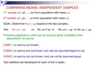
Independent Samples: Comparing Proportions. Lecture 41 Section 11.5 Fri, Apr 14, 2006. Comparing Proportions. We now wish to compare proportions between two populations. Normally, we would be measuring proportions for the same attribute.

E N D
Independent Samples: Comparing Proportions Lecture 41 Section 11.5 Fri, Apr 14, 2006
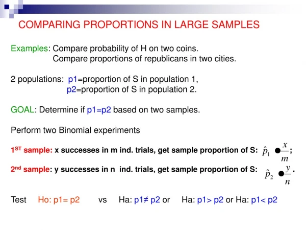
Comparing Proportions • We now wish to compare proportions between two populations. • Normally, we would be measuring proportions for the same attribute. • For example, we could measure the proportion of NC residents living below the poverty level and the proportion of VA residents living below the poverty level.
Examples • The “gender gap” – the proportion of men who vote Republican vs. the proportion of women who vote Republican. • The proportion of teenagers who smoked marijuana in 1995 vs. the proportion of teenagers who smoked marijuana in 2000.
Examples • The proportion of patients who recovered, given treatment A vs. the proportion of patients who recovered, given treatment B. • Treatment A could be a placebo.
Comparing proportions • To estimate the difference between population proportions p1 and p2, we need the sample proportions p1^ and p2^. • The difference p1^ – p2^ is an estimator of the difference p1 – p2.
Hypothesis Testing • See Example 11.8, p. 721 – Perceptions of the U.S.: Canadian versus French. • p1 = proportion of Canadians who feel positive about the U.S.. • p2 = proportion of French who feel positive about the U.S..
Hypothesis Testing • The hypotheses. • H0: p1 – p2 = 0 (i.e., p1 = p2) • H1: p1 – p2 > 0 (i.e., p1 > p2) • The significance level is = 0.05. • What is the test statistic? • That depends on the sampling distribution of p1^ – p2^.
The Sampling Distribution of p1^ – p2^ • If the sample sizes are large enough, then p1^ is N(p1, 1), where • Similarly, p2^ is N(p2, 2), where
The Sampling Distribution of p1^ – p2^ • The sample sizes will be large enough if • n1p1 5, and n1(1 – p1) 5, and • n2p2 5, and n2(1 – p2) 5.
The Sampling Distribution of p1^ – p2^ • Therefore, where
The Test Statistic • Therefore, the test statistic would be if we knew the values of p1 and p2. • We could estimate them with p1^ and p2^. • But there may be a better way…
Pooled Estimate of p • In hypothesis testing for the difference between proportions, typically the null hypothesis is H0: p1 = p2 • Under that assumption, p1^ and p2^ are both estimators of a common value (call it p).
Pooled Estimate of p • Rather than use either p1^ or p2^ alone to estimate p, we will use a “pooled” estimate. • The pooled estimate is the proportion that we would get if we pooled the two samples together.
The Standard Deviation of p1^ – p2^ • This leads to a better estimator of the standard deviation of p1^ – p2^.
Caution • If the null hypothesis does not say H0: p1 = p2 then we should not use the pooled estimate p^, but should use the unpooled estimate
The Test Statistic • So the test statistic is
The Value of the Test Statistic • Compute p^: • Now compute z:
The p-value, etc. • Compute the p-value: P(Z > 7.253) = 2.059 10-13. • Reject H0. • The data indicate that a greater proportion of Canadians than French have a positive feeling about the U.S.
Exercise 11.34 • Sample #1: 361 “Wallace” cars reveal that 270 have the sticker. • Sample #2: 178 “Humphrey” cars reveal that 154 have the sticker. • Do these data indicate that p1 p2?
Example • State the hypotheses. • H0: p1 = p2 • H1: p1p2 • State the level of significance. • = 0.05.
Example • Write the test statistic.
Example • Compute p1^, p2^, and p^.
Example • Now we can compute z.
Example • Compute the p-value. • p-value = 2 normalcdf(-E99, -3.126) = 2(0.0008861) = 0.001772. • The decision is to reject H0. • State the conclusion. • The data indicate that the proportion of Wallace cars that have the sticker is different from the proportion of Humphrey cars that have the sticker.
TI-83 – Testing Hypotheses Concerning p1^ – p2^ • Press STAT > TESTS > 2-PropZTest... • Enter • x1, n1 • x2, n2 • Choose the correct alternative hypothesis. • Select Calculate and press ENTER.
TI-83 – Testing Hypotheses Concerning p1^ – p2^ • In the window the following appear. • The title. • The alternative hypothesis. • The value of the test statistic z. • The p-value. • p1^. • p2^. • The pooled estimate p^. • n1. • n2.
Example • Work Exercise 11.34 using the TI-83.
Confidence Intervals for p1^ – p2^ • The formula for a confidence interval for p1^ – p2^ is • Caution: Note that we do not use the pooled estimate for p^.
TI-83 – Confidence Intervals for p1^ – p2^ • Press STAT > TESTS > 2-PropZInt… • Enter • x1, n1 • x2, n2 • The confidence level. • Select Calculate and press ENTER.
TI-83 – Confidence Intervals for p1^ – p2^ • In the window the following appear. • The title. • The confidence interval. • p1^. • p2^. • n1. • n2.
Example • Find a 95% confidence interval using the data in Exercise 11.34.