Kalman Filters
100 likes | 358 Vues
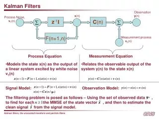
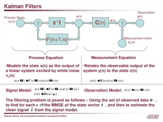
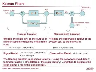
Kalman Filters. Observation y (n). x (n). Process Noise, v 1 (n). z -1 I. C (n). s (n). F(n+1,n). Measurement noise v 2 (n). Measurement Equation. Process Equation. Models the state x(n) as the output of a linear system excited by white noise v 1 (n).

Kalman Filters
E N D
Presentation Transcript
Kalman Filters Observation y(n) x(n) Process Noise, v1(n) z-1I C(n) s(n) F(n+1,n) Measurement noise v2(n) Measurement Equation Process Equation • Models the state x(n) as the output of a linear system excited by white noise v1(n) • Relates the observable output of the system y(n) to the state x(n) • Signal Model: Observation Model: • The filtering problem is posed as follows – Using the set of observed data , • to find for each the MMSE of the state vector , and then to estimate the clean signal from the signal model.
Unscented Kalman Filters (motivation… where Extended Kalman filters fail) • Nonlinear State Estimation • Predicting state vector, • Kalman gain, • Predicting observation • When propagating a GRV through a linear model (Kalman filtering), it is easy to compute the expectation E[ ] • However, if the same GRV passes through a nonlinear model, the resultant estimate may no longer be Gaussian – calculation of E[ ] is no longer easy! • It is in the calculation of E[ ] in the recursive filtering process that we now need to estimate the pdf of the propagating random vector F, H are (nonlinear) vector functions a Posteriori estimate Prediction of Innovation
Unscented Kalman Filters (motivation… where Extended Kalman filters fail) • Extended Kalman Filters (EKF) avoid this by linearizing the state-space equations and reducing the estimate equations to point estimates instead of expectations • The covariance matrices (P) are computed by linearizing the dynamic equations • In EKF, the state distributions are approximated by a GRV and propagated analytically through a ‘first-order linearization’ of the nonlinear system • - If the assumption of local linearity is violated, the resulting filter will be unstable • - The linearization process itself involves computations of Jacobians and Hessians (which is nontrivial for most systems)
The Unscented Transform • Problem statement: developing a method for calculating the statistics of a random variable which has undergone a nonlinear transformation • The intuition: It is easier to approximate a distribution than it is to approximate an arbitrary nonlinear transformation • Consider a nonlinearity • The Unscented transform chooses (deterministically) a set of ‘sigma’ points in the original (x) space which when mapped to the transformed (y) space will be capable of generating accurate sample means and covariance matrices in the transformed space • An accurate estimation of these allows us to use the Kalman filter in the usual setup, with the expectation values being replaced by sample means and covariance matrices as appropriate
The Unscented Transform (illustration) 0.2812 0.0046 0.0046 0.2014 Px 1.2692 0.0060 0.0060 0.8818 0.2709 0.0510 0.0510 0.1607 Py Py_ut
Unscented Kalman Filters (UKFs) • Instead of propagating a GRV through the “linearized” system, the UKF technique focuses on an efficient estimation of the statistics of the random vector being propagated through a nonlinear function • To compute the statistics of , we ‘cleverly’ sample this function using ‘deterministically’ chosen 2L+1 points about the mean of x • It can be proved that with these as sample points, the following ‘weighted’ sample means and covariance matrices will be equal to the true values • We use this set of equations to predict the states and observations in the nonlinear state-estimation model. The expected values E[ ] and the covariance matrices are replaced with these sample ‘weighted’ versions. Sigma Points
Unscented Kalman Filters (UKFs)… Algorithm development Augment the state vector to include the process and measurement noise and initialize the mean and covariance matrix of the augmented vector. Compute the sigma points about the previously estimated mean vector Compute the predicted value of the state vector and cov. matrix at time k Predict the current observation given previous observed samples (mapped from the sigma points) Compute the innovations covariance matrix, cross correlation matrix and hence the Kalman gain and update the current estimate of the state at time k Eric A. Wan and Rudolph van der Merwe, “The Unscented Kalman Filter for Nonlinear Estimation”
Unscented Kalman Filters (UKFs) vs. Particle Filters (PFs) • The unscented transformation in UKFs allows the calculation of accurate sample means and covariance matrices using a few ‘cleverly’ chosen samples • Particle filtering employs Monte-Carlo techniques to obtain an estimate of the statistics of the propagated random vector • The two techniques are very close conceptually • There is a subtle difference : in UKF based implementations, the sigma points for sampling are deterministically chosen whereas in PF based techniques, the sampling itself is done randomly • Particle Filtering is more accurate but this comes at the cost of complexity (introduced due to the need for Monte-Carlo simulations) • The complexity of UKF based implementations is about the same as that of regular Kalman filters