Kalman Filters and Dynamic Bayesian Networks
510 likes | 868 Vues
Source 1. Kalman Filters and Dynamic Bayesian Networks. Markoviana Reading Group Srinivas Vadrevu Arizona State University. Source 2. Introduction to Kalman Filters. CEE 6430: Probabilistic Methods in Hydroscienecs Fall 2008 Acknowledgements: Numerous sources on WWW, book, papers.

Kalman Filters and Dynamic Bayesian Networks
E N D
Presentation Transcript
Source 1 Kalman Filters andDynamic Bayesian Networks Markoviana Reading Group SrinivasVadrevu Arizona State University
Source 2 Introduction to Kalman Filters CEE 6430: Probabilistic Methods in Hydroscienecs Fall 2008 Acknowledgements: Numerous sources on WWW, book, papers
Outline • Introduction • Gaussian Distribution • Introduction • Examples (Linear and Multivariate) • Kalman Filters • General Properties • Updating Gaussian Distributions • One-dimensional Example • Notes about general case • Applicability of Kalman Filtering • Dynamic Bayesian Networks (DBNs) • Introduction • DBNs and HMMs • DBNs and HMMs • Constructing DBNs Markoviana Reading Group: Week3
A “Hydro” Example • Suppose you have a hydrologic model that predicts river water level every hour (using the usual inputs). • You know that your model is not perfect and you don’t trust it 100%. So you want to send someone to check the river level in person. • However, the river level can only be checked once a day around noon and not every hour. • Furthermore, the person who measures the river level can not be trusted 100% either. • So how do you combine both outputs of river level (from model and from measurement) so that you get a ‘fused’ and better estimate? – Kalman filtering
What is a Filter by the way? • Other applications of Kalman Filtering (or Filtering in general): • Your Car GPS (predict and update location) • Surface to Air Missile (hitting the target) • Ship or Rocket navigation (Appollo 11 used some sort of filtering to make sure it didn’t miss the Moon!)
The Problem in General (let’s get a little more technical) • System state cannot be measured directly • Need to estimate “optimally” from measurements Black Box System Error Sources Sometimes the system state and the measurement may be two different things (not like river level example) External Controls System System State (desired but not known) Optimal Estimate of System State Observed Measurements Measuring Devices Estimator Measurement Error Sources
What is a Kalman Filter? • Recursive data processing algorithm • Generates optimal estimate of desired quantities given the set of measurements • Optimal? • For linear system and white Gaussian errors, Kalman filter is “best” estimate based on all previous measurements • For non-linear system optimality is ‘qualified’ • Recursive? • Doesn’t need to store all previous measurements and reprocess all data each time step
Conceptual Overview • Simple example to motivate the workings of the Kalman Filter • The essential equations you need to know (Kalman Filtering for Dummies!) • Examples: Prediction and Correction
Conceptual Overview • Lost on the 1-dimensional line (imagine that you are guessing your position by looking at the stars using sextant) • Position – y(t) • Assume Gaussian distributed measurements y
Conceptual Overview State space – position Measurement - position Sextant is not perfect • Sextant Measurement at t1: Mean = z1 and Variance = z1 • Optimal estimate of position is: ŷ(t1) = z1 • Variance of error in estimate: 2x(t1) = 2z1 • Boat in same position at time t2 - Predicted position is z1
Conceptual Overview prediction ŷ-(t2) State (by looking at the stars at t2) Measurement usign GPS z(t2) • So we have the prediction ŷ-(t2) • GPS Measurement at t2: Mean = z2 and Variance = z2 • Need to correct the prediction by Sextant due to measurement to get ŷ(t2) • Closer to more trusted measurement – should we do linear interpolation?
Conceptual Overview prediction ŷ-(t2) Kalman filter helps you fuse measurement and prediction on the basis of how much you trust each (I would trust the GPS more than the sextant) corrected optimal estimate ŷ(t2) measurement z(t2) • Corrected mean is the new optimal estimate of position (basically you have ‘updated’ the predicted position by Sextant using GPS • New variance is smaller than either of the previous two variances
Conceptual Overview(The Kalman Equations) • Lessons so far: Make prediction based on previous data - ŷ-, - Take measurement – zk, z Optimal estimate (ŷ) = Prediction + (Kalman Gain) * (Measurement - Prediction) Variance of estimate = Variance of prediction * (1 – Kalman Gain)
Conceptual Overview What if the boat was now moving? ŷ(t2) Naïve Prediction (sextant) ŷ-(t3) • At time t3, boat moves with velocity dy/dt=u • Naïve approach: Shift probability to the right to predict • This would work if we knew the velocity exactly (perfect model)
Conceptual Overview Naïve Prediction ŷ-(t3) But you may not be so sure about the exact velocity ŷ(t2) Prediction ŷ-(t3) • Better to assume imperfect model by adding Gaussian noise • dy/dt = u + w • Distribution for prediction moves and spreads out
Conceptual Overview Corrected optimal estimate ŷ(t3) Updated Sextant position using GPS Measurement z(t3) GPS Prediction ŷ-(t3) Sextant • Now we take a measurement at t3 • Need to once again correct the prediction • Same as before
Conceptual Overview • Lessons learnt from conceptual overview: • Initial conditions (ŷk-1 and k-1) • Prediction (ŷk-, k-) • Use initial conditions and model (eg. constant velocity) to make prediction • Measurement (zk) • Take measurement • Correction (ŷk , k) • Use measurement to correct prediction by ‘blending’ prediction and residual – always a case of merging only two Gaussians • Optimal estimate with smaller variance
Blending Factor • If we are sure about measurements: • Measurement error covariance (R) decreases to zero • K decreases and weights residual more heavily than prediction • If we are sure about prediction • Prediction error covariance P-k decreases to zero • K increases and weights prediction more heavily than residual
Correction (Measurement Update) Prediction (Time Update) (1) Compute the Kalman Gain (1) Project the state ahead K = P-kHT(HP-kHT + R)-1 ŷ-k = Ayk-1 + Buk (2) Update estimate with measurement zk (2) Project the error covariance ahead ŷk = ŷ-k + K(zk - H ŷ-k ) P-k = APk-1AT + Q (3) Update Error Covariance Pk = (I - KH)P-k The set of Kalman Filtering Equations in Detail
Assumptions behind Kalman Filter • The model you use to predict the ‘state’ needs to be a LINEAR function of the measurement (so how do we use non-linear rainfall-runoff models?) • The model error and the measurement error (noise) must be Gaussian with zero mean
HMMs and Kalman Filters • Hidden Markov Models (HMMs) • Discrete State Variables • Used to model sequence of events • Kalman Filters • Continuous State Variables, with Gaussian Distribution • Used to model noisy continuous observations • Examples • Predict the motion of a bird through dense jungle foliage at dusk • Predict the direction of the missile through intermittent radar movement observations Markoviana Reading Group: Week3
Gaussian (Normal) Distribution • Central Limit Theorem: The sum of n statistical independent random variables converges for n ∞ towards the Gaussian distribution (Applet Illustration) • Unlike the binomial and Poisson distribution, the Gaussian is a continuous distribution: • = mean of distribution (also at the same place as mode and median) • 2 = variance of distribution • y is a continuous variable (-∞y∞ • Gaussian distribution is fully defined by its mean and variance Markoviana Reading Group: Week3
Gaussian Distribution: Examples • Linear Gaussian Distribution • Mean, and Variance, • Multivariate Gaussian Distribution • For 3 random variables • Mean, = [m1 m2 m3] • Covariance Matrix, Sigma = [ v11 v12 v13 v21 v22 v23 v31 v32 v33 ] Markoviana Reading Group: Week3
Kalman Filters: General Properties • Estimate the state and the covariance of the state at any time T, given observations, xT = {x1, …, xT} • E.g., Estimate the state (location and velocity) of airplane and its uncertainty, given some measurements from an array of sensors • The probability of interest is P(yt|xT) • Filtering the state T = current time, t • Predicting the state T < current time, t • Smoothing the state T > current time, t Markoviana Reading Group: Week3
Gaussian Noise & Example • Next State is linear function of current state, plus some Gaussian noise • Position Update: • Gaussian Noise: Markoviana Reading Group: Week3
Updating Gaussian Distributions • Linear Gaussian family of distributions remains closed under standard Bayesian network operations ( this means we end up with Gaussian distributions – a very nice property.) • One-step predicted distribution • Current distribution P(Xt|e1:t) is Gaussian • Transition model P(Xt+1|xt) is linear Gaussian • The updated distribution • Predicted distribution P(Xt+1|e1:t) is Gaussian • Sensor model P(et+1|Xt+1) is linear Gaussian • Filtering and Prediction (From 15.2): Markoviana Reading Group: Week3
One-dimensional Example • Update Rule (Derivations from Russel & Norvig) • Compute new mean and covariance matrix from the previous mean and covariance matrix • Variance update is independent of the observation • Another variation of the update rule (from Max Welling, Caltech) - t+1 is weighted mean of new observation Zt+1 and the old meant • Observation unreliable 2z is large (more attention to old mean) • Old mean unreliable 2t is large (more attention to observation) • - 2 is variance or uncertainty, K is the Kalman gain • K = 0 no attention to measurement • - K = 1 complete attention to measurement Markoviana Reading Group: Week3
The General Case • Multivariate Gaussian Distribution • Exponent is a quadratic function of the random variables xi in x • Temporal model with Kalman filtering • F: linear transition model • H: linear sensor model • Sigma_x: transition noise covariance • Sigma_z: sensor noise covariance • Update equations for mean and covariance • Kt+1: the Kalman gain matrix • Ft: predicted state at t+1 • HFt: the predicted observation • Zt+1 – HFt: error in predicted observation Markoviana Reading Group: Week3
Illustration Markoviana Reading Group: Week3
Applicability of Kalman Filtering • Popular applications • Navigation, guidance, radar tracking, sonar ranging, satellite orbit computation, stock price prediction, landing of Eagle on Moon, gyroscopes in airplanes, etc. • Extended Kalman Filters (EKF) can handle Nonlinearities in Gaussian distributions • Model the system as locally linear in xt in the region of xt = t • Works well for smooth, well-behaved systems • Switching Kalman Filters: multiple Kalman filters in parallel, each using different model of the system • A weighted sum of predictions used Markoviana Reading Group: Week3
Applicability of Kalman Filters Markoviana Reading Group: Week3
Dynamic Bayesian Networks • Directed graphical models of stochastic processes • Extend HMMs by representing hidden (and observed) state in terms of state variables, with possible complex interdependencies • Any number of state variables and evidence variables • Dynamic or Temporal Bayesian Network??? • Model structure does not change over time • Parameters do not change over time • Extra hidden nodes can be added (mixture of models) Markoviana Reading Group: Week3
DBNs and HMMs • HMM as a DBN • Single state variable and single evidence variable • Discrete variable DBN as an HMM • Combine all state variables in DBN into a single state variable (with all possible values of individual state variables) • Efficient Representation (with 20 boolean state variables, DBN needs 160 probabilities, whereas HMM needs roughly a trillion probabilities) • Analogous to Ordinary Bayesian Networks vs Fully Tabulated Joint Distributions Markoviana Reading Group: Week3
DBNs and Kalman Filters • Kalman filter as a DBN • Continuous variables and linear Gaussian conditional distributions • DBN as a Kalman Filter • Not possible • DBN allows any arbitrary distributions • Lost keys example Markoviana Reading Group: Week3
Constructing DBNs • Required information • Prior distributions over state variables P(X0) • The transition model P(Xt+1|Xt) • The sensor model P(Et|Xt) Markoviana Reading Group: Week3