Download
1 / 51
510 likes | 680 Vues
I/O Systems. interrupts. Processor. Cache. Memory - I/O Bus. Main Memory. I/O Controller. I/O Controller. I/O Controller. Graphics. Disk. Disk. Network. Driven by the prevailing computing paradigm 1950s: migration from batch to on-line processing

E N D
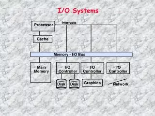
I/O Systems interrupts Processor Cache Memory - I/O Bus Main Memory I/O Controller I/O Controller I/O Controller Graphics Disk Disk Network
Driven by the prevailing computing paradigm 1950s: migration from batch to on-line processing 1990s: migration to ubiquitous computing computers in phones, books, cars, video cameras, … nationwide fiber optical network with wireless tails Effects on storage industry: Embedded storage smaller, cheaper, more reliable, lower power Data utilities high capacity, hierarchically managed storage Storage Technology Drivers
Disk Basics Disk History Disk options in 2000 Disk fallacies and performance FLASH Tapes RAID Outline
Several platters, with information recorded magnetically on both surfaces (usually) Inner Track Outer Track Sector Head Arm Platter Actuator Disk Device Terminology • Bits recorded in tracks, which in turn divided into sectors (e.g., 512 Bytes) • Actuator moves head (end of arm,1/surface) over track (“seek”), select surface, wait for sector rotate under head, then read or write • “Cylinder”: all tracks under heads
{ Platters (12) Photo of Disk Head, Arm, Actuator Spindle Arm Head Actuator
Disk Latency = Seek Time + Rotation Time + Transfer Time + Controller Overhead Seek Time? depends no. tracks move arm, seek speed of disk Rotation Time? depends on speed disk rotates, how far sector is from head Transfer Time? depends on data rate (bandwidth) of disk (bit density), size of request Disk Device Performance Inner Track Outer Track Sector Head Controller Arm Spindle Platter Actuator
Average distance sector from head? 1/2 time of a rotation 10000 Revolutions Per Minute 166.67 Rev/sec 1 revolution = 1/ 166.67 sec 6.00 milliseconds 1/2 rotation (revolution) 3.00 ms Average no. tracks move arm? Sum all possible seek distances from all possible tracks / # possible Assumes average seek distance is random Disk industry standard benchmark Disk Device Performance
To keep things simple, orginally kept same number of sectors per track Since outer track longer, lower bits per inch Competition decided to keep BPI the same for all tracks (“constant bit density”) More capacity per disk More of sectors per track towards edge Since disk spins at constant speed, outer tracks have faster data rate Bandwidth outer track 1.7X inner track! Inner track highest density, outer track lowest, so not really constant 2.1X length of track outer / inner, 1.7X bits outer / inner Data Rate: Inner vs. Outer Tracks
Purpose: Long-term, nonvolatile storage Large, inexpensive, slow level in the storage hierarchy Characteristics: Seek Time (~8 ms avg) positional latency rotational latency Transfer rate 10-40 MByte/sec Blocks Capacity Gigabytes Quadruples every 2 years (aerodynamics) Response time = Queue + Controller + Seek + Rot + Xfer Service time Devices: Magnetic Disks Track Sector Cylinder Platter Head 7200 RPM = 120 RPS => 8 ms per rev ave rot. latency = 4 ms 128 sectors per track => 0.25 ms per sector 1 KB per sector => 16 MB / s
Capacity + 100%/year (2X / 1.0 yrs) Transfer rate (BW) + 40%/year (2X / 2.0 yrs) Rotation + Seek time – 8%/ year (1/2 in 10 yrs) MB/$ > 100%/year (2X / 1.0 yrs) Fewer chips + areal density Disk Performance Model /Trends
181.6 GB, 3.5 inch disk 12 platters, 24 surfaces 24,247 cylinders 7,200 RPM; (4.2 ms avg. latency) 7.4/8.2 ms avg. seek (r/w) 64 to 35 MB/s (internal) 0.1 ms controller time 10.3 watts (idle) Latency = Queuing Time + Controller time + Seek Time + Rotation Time + Size / Bandwidth { per access + per byte State of the Art: Barracuda 180 Track Sector Cylinder Track Buffer Arm Platter Head source: www.seagate.com
Calculate time to read 64 KB (128 sectors) for Barracuda 180 X using advertised performance; sector is on outer track Disk latency = average seek time + average rotational delay + transfer time + controller overhead = 7.4 ms + 0.5 * 1/(7200 RPM) + 64 KB / (65 MB/s) + 0.1 ms = 7.4 ms + 0.5 /(7200 RPM/(60000ms/M)) + 64 KB / (65 KB/ms) + 0.1 ms = 7.4 + 4.2 + 1.0 + 0.1 ms = 12.7 ms Disk Performance Example (will fix later)
Bits recorded along a track Metric is Bits Per Inch (BPI) Number of tracks per surface Metric is Tracks Per Inch (TPI) Disk Designs Brag about bit density per unit area Metric is Bits Per Square Inch Called Areal Density Areal Density =BPI x TPI Areal Density
Areal Density • Areal Density =BPI x TPI • Change slope 30%/yr to 60%/yr about 1991
MBits per square inch: DRAM as % of Disk over time 9 v. 22 Mb/si 470 v. 3000 Mb/si 0.2 v. 1.7 Mb/si source: New York Times, 2/23/98, page C3, “Makers of disk drives crowd even mroe data into even smaller spaces”
1956 IBM Ramac — early 1970s Winchester Developed for mainframe computers, proprietary interfaces Steady shrink in form factor: 27 in. to 14 in Form factor and capacity drives market, more than performance 1970s: Mainframes 14 inch diameter disks 1980s: Minicomputers,Servers 8”,5 1/4” diameter PCs, workstations Late 1980s/Early 1990s: Mass market disk drives become a reality industry standards: SCSI, IPI, IDE Pizzabox PCs 3.5 inch diameter disks Laptops, notebooks 2.5 inch disks Palmtops didn’t use disks, so 1.8 inch diameter disks didn’t make it 2000s: 1 inch for cameras, cell phones? Historical Perspective
Disk History Data density Mbit/sq. in. Capacity of Unit Shown Megabytes 1973: 1. 7 Mbit/sq. in 140 MBytes 1979: 7. 7 Mbit/sq. in 2,300 MBytes source: New York Times, 2/23/98, page C3, “Makers of disk drives crowd even more data into even smaller spaces”
Disk History 1989: 63 Mbit/sq. in 60,000 MBytes 1997: 1450 Mbit/sq. in 2300 MBytes 1997: 3090 Mbit/sq. in 8100 MBytes source: New York Times, 2/23/98, page C3, “Makers of disk drives crowd even mroe data into even smaller spaces”
1 inch disk drive! • 2000 IBM MicroDrive: • 1.7” x 1.4” x 0.2” • 1 GB, 3600 RPM, 5 MB/s, 15 ms seek • Digital camera, PalmPC? • 2006 MicroDrive? • 9 GB, 50 MB/s! • Assuming it finds a niche in a successful product • Assuming past trends continue
Disk Characteristics in 2000 $828 $447 $435
Manufacturers needed standard for fair comparison (“benchmark”) Calculate all seeks from all tracks, divide by number of seeks => “average” Real average would be based on how data laid out on disk, where seek in real applications, then measure performance Usually, tend to seek to tracks nearby, not to random track Rule of Thumb: observed average seek time is typically about 1/4 to 1/3 of quoted seek time (i.e., 3X-4X faster) Barracuda 180 X avg. seek: 7.4 ms 2.5 ms Fallacy: Use Data Sheet “Average Seek” Time
Manufacturers quote the speed off the data rate off the surface of the disk Sectors contain an error detection and correction field (can be 20% of sector size) plus sector number as well as data There are gaps between sectors on track Rule of Thumb: disks deliver about 3/4 of internal media rate (1.3X slower) for data For example, Barracuda 180X quotes 64 to 35 MB/sec internal media rate 47 to 26 MB/sec external data rate (74%) Fallacy: Use Data Sheet Transfer Rate
Calculate time to read 64 KB for UltraStar 72 again, this time using 1/3 quoted seek time, 3/4 of internal outer track bandwidth; (12.7 ms before) Disk latency = average seek time + average rotational delay + transfer time + controller overhead = (0.33 * 7.4 ms) + 0.5 * 1/(7200 RPM) + 64 KB / (0.75 * 65 MB/s) + 0.1 ms = 2.5 ms + 0.5 /(7200 RPM/(60000ms/M)) + 64 KB / (47 KB/ms) + 0.1 ms = 2.5 + 4.2 + 1.4 + 0.1 ms = 8.2 ms (64% of 12.7) Disk Performance Example
Continued advance in capacity (60%/yr) and bandwidth (40%/yr) Slow improvement in seek, rotation (8%/yr) Time to read whole disk Year Sequentially Randomly (1 sector/seek) 1990 4 minutes 6 hours 2000 12 minutes 1 week(!) 3.5” form factor make sense in 5 yrs? What is capacity, bandwidth, seek time, RPM? Assume today 80 GB, 30 MB/sec, 6 ms, 10000 RPM Future Disk Size and Performance
Compact Flash Cards Intel Strata Flash 16 Mb in 1 square cm. (.6 mm thick) 100,000 write/erase cycles. Standby current = 100uA, write = 45mA Compact Flash 256MB~=$120 512MB~=$542 Transfer @ 3.5MB/s IBM Microdrive 1G~370 Standby current = 20mA, write = 250mA Efficiency advertised in wats/MB VS. Disks Nearly instant standby wake-up time Random access to data stored Tolerant to shock and vibration (1000G of operating shock) What about FLASH
Tape vs. Disk • • Longitudinal tape uses same technology as • hard disk; tracks its density improvements • Disk head flies above surface, tape head lies on surface • Disk fixed, tape removable • • Inherent cost-performance based on geometries: • fixed rotating platters with gaps • (random access, limited area, 1 media / reader) • vs. • removable long strips wound on spool • (sequential access, "unlimited" length, multiple / reader) • • Helical Scan (VCR, Camcoder, DAT) • Spins head at angle to tape to improve density
Tape wear out: Helical 100s of passes to 1000s for longitudinal Head wear out: 2000 hours for helical Both must be accounted for in economic / reliability model Bits stretch Readers must be compatible with multiple generations of media Long rewind, eject, load, spin-up times; not inherent, just no need in marketplace Designed for archival Current Drawbacks to Tape
6000 x 50 GB 9830 tapes = 300 TBytes in 2000 (uncompressed) Library of Congress: all information in the world; in 1992, ASCII of all books = 30 TB Exchange up to 450 tapes per hour (8 secs/tape) 1.7 to 7.7 Mbyte/sec per reader, up to 10 readers Automated Cartridge System: StorageTek Powderhorn 9310 7.7 feet 8200 pounds,1.1 kilowatts 10.7 feet
Getting books today as quaint as the way I learned to program punch cards, batch processing wander thru shelves, anticipatory purchasing Cost $1 per book to check out $30 for a catalogue entry 30% of all books never checked out Write only journals? Digital library can transform campuses Library vs. Storage
Investment in research: 90% of disks shipped in PCs; 100% of PCs have disks ~0% of tape readers shipped in PCs; ~0% of PCs have disks Before, N disks / tape; today, N tapes / disk 40 GB/DLT tape (uncompressed) 80 to 192 GB/3.5" disk (uncompressed) Cost per GB: In past, 10X to 100X tape cartridge vs. disk Jan 2001: 40 GB for $53 (DLT cartridge), $2800 for reader $1.33/GB cartridge, $2.03/GB 100 cartridges + 1 reader ($10995 for 1 reader + 15 tape autoloader, $10.50/GB) Jan 2001: 80 GB for $244 (IDE,5400 RPM), $3.05/GB Will $/GB tape v. disk cross in 2001? 2002? 2003? Storage field is based on tape backup; what should we do? Discussion if time permits? Whither tape?
Use Arrays of Small Disks? • Katz and Patterson asked in 1987: • Can smaller disks be used to close gap in performance between disks and CPUs? Conventional: 4 disk designs 3.5” 5.25” 10” 14” High End Low End Disk Array: 1 disk design 3.5”
Advantages of Small Formfactor Disk Drives Low cost/MB High MB/volume High MB/watt Low cost/Actuator Cost and Environmental Efficiencies
Replace Small Number of Large Disks with Large Number of Small Disks! (1988 Disks) IBM 3390K 20 GBytes 97 cu. ft. 3 KW 15 MB/s 600 I/Os/s 250 KHrs $250K x70 23 GBytes 11 cu. ft. 1 KW 120 MB/s 3900 IOs/s ??? Hrs $150K IBM 3.5" 0061 320 MBytes 0.1 cu. ft. 11 W 1.5 MB/s 55 I/Os/s 50 KHrs $2K Capacity Volume Power Data Rate I/O Rate MTTF Cost 9X 3X 8X 6X Disk Arrays have potential for large data and I/O rates, high MB per cu. ft., high MB per KW, but what about reliability?
Array Reliability • Reliability of N disks = Reliability of 1 Disk ÷ N • 50,000 Hours ÷ 70 disks = 700 hours • Disk system MTTF: Drops from 6 years to 1 month! • • Arrays (without redundancy) too unreliable to be useful! Hot spares support reconstruction in parallel with access: very high media availability can be achieved
Files are "striped" across multiple disks Redundancy yields high data availability Availability: service still provided to user, even if some components failed Disks will still fail Contents reconstructed from data redundantly stored in the array Capacity penalty to store redundant info Bandwidth penalty to update redundant info Redundant Arrays of (Inexpensive) Disks
Redundant Arrays of Inexpensive DisksRAID 1: Disk Mirroring/Shadowing recovery group • • Each disk is fully duplicated onto its “mirror” • Very high availability can be achieved • • Bandwidth sacrifice on write: • Logical write = two physical writes • • Reads may be optimized • • Most expensive solution: 100% capacity overhead • (RAID 2 not interesting, so skip)
10010011 11001101 10010011 . . . P 1 0 1 0 0 0 1 1 1 1 0 0 1 1 0 1 1 0 1 0 0 0 1 1 1 1 0 0 1 1 0 1 logical record Striped physical records Redundant Array of Inexpensive Disks RAID 3: Parity Disk P contains sum of other disks per stripe mod 2 (“parity”) If disk fails, subtract P from sum of other disks to find missing information
Sum computed across recovery group to protect against hard disk failures, stored in P disk Logically, a single high capacity, high transfer rate disk: good for large transfers Wider arrays reduce capacity costs, but decreases availability 33% capacity cost for parity in this configuration RAID 3
RAID 3 relies on parity disk to discover errors on Read But every sector has an error detection field Rely on error detection field to catch errors on read, not on the parity disk Allows independent reads to different disks simultaneously Inspiration for RAID 4
Stripe Redundant Arrays of Inexpensive Disks RAID 4: High I/O Rate Parity Increasing Logical Disk Address D0 D1 D2 D3 P Insides of 5 disks D7 P D4 D5 D6 D8 D9 D10 P D11 Example: small read D0 & D5, large write D12-D15 D12 D13 P D14 D15 D16 D17 D18 D19 P D20 D21 D22 D23 P . . . . . . . . . . . . . . . Disk Columns
RAID 4 works well for small reads Small writes (write to one disk): Option 1: read other data disks, create new sum and write to Parity Disk Option 2: since P has old sum, compare old data to new data, add the difference to P Small writes are limited by Parity Disk: Write to D0, D5 both also write to P disk D0 D1 D2 D3 P D7 P D4 D5 D6 Inspiration for RAID 5
Redundant Arrays of Inexpensive Disks RAID 5: High I/O Rate Interleaved Parity Increasing Logical Disk Addresses D0 D1 D2 D3 P Independent writes possible because of interleaved parity D4 D5 D6 P D7 D8 D9 P D10 D11 D12 P D13 D14 D15 Example: write to D0, D5 uses disks 0, 1, 3, 4 P D16 D17 D18 D19 D20 D21 D22 D23 P . . . . . . . . . . . . . . . Disk Columns
Problems of Disk Arrays: Small Writes RAID-5: Small Write Algorithm 1 Logical Write = 2 Physical Reads + 2 Physical Writes D0 D1 D2 D0' D3 P old data new data old parity (1. Read) (2. Read) XOR + + XOR (3. Write) (4. Write) D0' D1 D2 D3 P'
System Availability: Orthogonal RAIDs Array Controller String Controller . . . String Controller . . . String Controller . . . String Controller . . . String Controller . . . String Controller . . . Data Recovery Group: unit of data redundancy Redundant Support Components: fans, power supplies, controller, cables End to End Data Integrity: internal parity protected data paths
System-Level Availability host host Fully dual redundant I/O Controller I/O Controller Array Controller Array Controller . . . . . . . . . Goal: No Single Points of Failure . . . . . . . . . with duplicated paths, higher performance can be obtained when there are no failures Recovery Group
RAID-I (1989) Consisted of a Sun 4/280 workstation with 128 MB of DRAM, four dual-string SCSI controllers, 28 5.25-inch SCSI disks and specialized disk striping software Today RAID is $19 billion dollar industry, 80% nonPC disks sold in RAIDs Berkeley History: RAID-I
Summary: RAID Techniques: Goal was performance, popularity due to reliability of storage 1 0 0 1 0 0 1 1 1 0 0 1 0 0 1 1 • Disk Mirroring, Shadowing (RAID 1) Each disk is fully duplicated onto its "shadow" Logical write = two physical writes 100% capacity overhead 1 0 0 1 0 0 1 1 0 0 1 1 0 0 1 0 1 1 0 0 1 1 0 1 1 0 0 1 0 0 1 1 • Parity Data Bandwidth Array (RAID 3) Parity computed horizontally Logically a single high data bw disk • High I/O Rate Parity Array (RAID 5) Interleaved parity blocks Independent reads and writes Logical write = 2 reads + 2 writes