Quantitative genetics and breeding theory
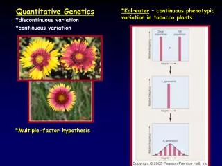
750 likes | 1.09k Vues
Quantitative genetics and breeding theory. Mini-course by Dag Lindgren Dag.Lindgren@genfys.slu.se Umeå 03-03-10-12, Raleigh, USA. Acknowledgements to Darius Danusevicius for assistance in the lay out. Message from a senior and old professor of Forest Genetics.

Quantitative genetics and breeding theory
E N D
Presentation Transcript
Quantitative genetics and breeding theory Mini-course by Dag Lindgren Dag.Lindgren@genfys.slu.se Umeå 03-03-10-12, Raleigh, USA Acknowledgements to Darius Danusevicius for assistance in the lay out
Message from a senior and old professor of Forest Genetics At least one week attention on the concepts behind TBT is needed each five years: • For all who call themselves forest tree breeders • For all who get the doctors title in forest genetics in the future • For most professional forest geneticists
General website: http://www.genfys.slu.se/staff/dagl/ In particular “Tree Breeding Tools” (TBT) http://www.genfys.slu.se/staff/dagl/Breed_Home_Page/ The start of this course is almost identically given at http://www.genfys.slu.se/staff/dagl/Breed_Home_Page/Tutorials/Quant_Gen/Kurs01A_for_site.htm This mini-course is much my personal view of the use of quantitative genetics applied to forest tree breeding. Other “schools” have other emphases. Some concepts are established. Other I, or collaborators, have coined.Most, but not all, stuff presented is published somewhere,
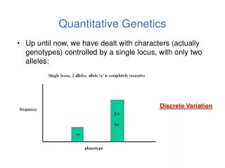
Common assumptions • One character – but may be composite! • Diploid zygotes and haploid gametes Meiosis Haploid gametes Diploid zygote Mitosis Diploid progeny
Semantics • Many misunderstandings and conflicts are semantic (a matter of definitions) • Important to speak the same language – and use the same symbols – at least within group. The second best is to understand that people speak different languages. No it’s a plant This is a tree
Gain(BV) Inbreeding Coancestry Gene diversity Cost Environments Technique Genetic parameters Interactions The art of breeding is combining a lot of things in a good way!
To do that effectively, we must have quantitative concepts and measures To optimize, a quantitative measure must be defined and maximized!
Some concepts useful for quantitative genetics Identical by descent(IBD) means that genes at the same locus are copies of the same original gene in some ancestor. The chance that both homologous genes in the same zygote are identical by descent is called inbreeding (F) (or coefficient of inbreeding).
Coancestry(, f) between pair of individuals is the probability that genes, taken at random from each of the concerned individuals, are identical by descent (=coefficient of coancestry). A quantification of relatedness. We will widen that concept! Self-coancestry: An individual's coancestry with itself is 0.5(1+F). This can be realised e.g. by considering that coancestry in the previous generation becomes inbreeding in next, and then consider selfing. If two individuals mate, their coancestry becomes the inbreeding of their offspring. Note that inbreeding and coancestry are relative to a situation with no inbreeding or relatedness.
Founder population is the starting point of calculations. If all inbreeding and coancestry of the founder population is known, inbreeding and coancestry can be calculated from a pedigree. It is usually practical and convenient to set inbreeding and coancestry to zero in the "wild forest" (or source population) and see the founders (plus trees) as a sample from the wild forest. Inbreeding and coancestry are relative to some real or imaginary "base" or "reference" or "source" population. Most conveniently this is the founder population or the wild forest. Self-coancestry: An individual's coancestry with itself is 0.5(1+F). This can be realised e.g. by considering that coancestry in the previous generation becomes inbreeding in next, and then consider selfing.
Gene poolmeans all genes in a population. It is convenient to consider genes at one locus. The gene pool is independent on how (or if) a population is organised in zygotes. Gene pool A population with N zygotes has 2N genes in the gene pool ....2N e.g 2 zygotes with 4 genes in the picture above
....2N Each gene has the frequency 1/2N Arrows = sampling with replacement (or infinite copies of each gene) Probability to sample the same gene twice is 1/2N Probability that different genes will be sampled is (1-0.5/N).
f= coancestry Genes can be IBD (identical by descent). The probability is the coancestry (f).
f = coancestry Individual A Individual B The probability that the genes in two specific individuals are IBD is the coancestry between these two individuals. The gene pool is often structured in individuals
For self-coancestry, the genes need not to be different. If they are different f=F; if the same f=1; average f=(1+F)/2. The probability that the two different genes in the same zygote are IBD is the coefficient of inbreeding (F). F= inbreeding
Different mechanisms genes sampled from a population may be IBD: 1. The same gene sampled twice (drift); 2. The genes are homologous genes from the same individual (inbreeding), 3. The genes originate from different individuals (relatedness).
Pair-wise coancestries arranged in a coancestry matrix We denote a certain value by f2,1=0.25 Symmetric, thusf2,1= f1,2 The values along the diagonal (self-coancestries) appear only once. Coefficient of relationship are often arranged in such a matrix, (numerator matrix), in absence of inbreeding these values are double as large.
Examples of coancestry Relative Coancestry (f,) Unrelated 0 Half sibs 0.125 Full sibs 0.25 Parent-offspring 0.25 Cousin 0.0625 Itself (self-coancestry) 0.5 Coancestries are probabilities, thus 0 f 1.
mother sister aunt uncle cousin What is the average relatedness (group coancestry) of this ”family”? Group coancestry
Group coancestry Let's put all homologous genes in a big pool and select two (at random with replacement). The probability that two are IBD we define as group coancestry. (, this term was introduced by Cockerham 1967). f To get overall probability; average over all individual probabilities, f. Group coancestry equals the average of all N2 coancestry values among all combinations of the N individuals in a population (or the average of all 4N2 combinations of individual genes). We could as well define group coancestry as this average, the advantage of the probabilistic definition appears in more complex situations.
Sum of the 9 values in matrix= 2.5; Average = group coancestry = 2.5/9 = 0.278 Note that self-coancestries appear once, while other coancestries appear twice (reciprocals).
If all individuals in a population are related in the same pattern, it is enough to calculate the N coancestries for a single individual. Self-coancestry is the group coancestry for a population with a single member. All members in a full sib family have equal coancestries to all other individuals. Thus it is enough to construct the coancestry matrix for full sib families (and make some thinking). Group coancestry depends on relatedness, not how unitinggametes are arranged. A brother is equally related to his brother as to his sister, in spite of that his gametes are able to unite only with those of his sister.
Group coancestry for families Family size = n, no inbreeding
Cross-coancestry and Self-coancestry The term cross-coancestry is used here for the average of all coancestry-values among different individuals excepting self-coancestry. Using “Coancestry” for “average cross-coancestry” invites to misunderstandings. Group-coancestry can be separated in two types: Self-coancestry and cross-coancestry.
Cross-coancestry, Inbreeding and Group Coancestry relations • A population can be described by: • Inbreeding (or average self-coancestry) • Group-coancestry • Average Cross-coancestry • If two are known, the third can be derived
Using the following relationships, group coancestry and average cross-coancestry can be derived where: = group coancestry; N = individuals; f = average cross-coancestry; F = average inbreeding.
Linking generations Group coancestry changes at generation shifts can be calculated retrospectively from a known pedigree linking to the founders. Future group coancestry can be calculated with knowledge or assumptions about future pedigrees. For other cases predictions may be made, but this is often far from trivial. Note that there may be doubt if assumptions are realistic (neutral selection, many genes with infinitesimal action etc.)
The link between generations is the gametes. parents offspring The gene pool of the offspring is identical to the gene pool of the successful gametes of the parents.
2Nparents parents 2Noffspring offspring 2Noffspring offspring Consider a pair of genes, which may equivalently be regarded as in offspring zygotes or in parental successful gametes! A pair of genes in offspring may be IBD as they are copies of the same gene in the parent population. This may happen if a parent has more than one offspring.
A pair of genes may originate from homogenous genes of the same parental zygote in the parental generation, if that was inbred, the considered genes may be IBD. F 2Nparents parents 2Noffspring offspring Different gametes from a parent get coancestry (1+Fparent)/2 Sibs sharing that parent (half sib) get coancestry (1+Fparent)/8.
f If the considered gene pair originates from different parents, the coancestry will be fparent. 2Nparents parents 2Noffspring offspring
IBD may occur by the following mechanisms: 1. The same gene in the current generation is sampled twice, 2. The genes are copies of the same gene in the parental generation, 3. The genes origin from homologous genes in the same inbred parent, 4. The genes come from different, but related, parents.
Group coancestry and gene diversity • Group coancestry is the probability that two genes are IBD; • Diversity means that things are different; • Gene Diversity means that genes are different. • Evidently 1 - group coancestry is the probability that the genes are non-identical, thus diverse.
GD = 1 - group coancestry is the probability that the genes are non-identical, thus diverse. GD is Gene Diversity! Group coancestry is a measure of gene diversity lost! That seems to be something worth knowing!
This way of thinking sees all genes in the source (reference) populations as unique (“tagged”). GD is similar to expected average heterozygosity (the chance that two genes are different). Group coancestry based measures are (like inbreeding) relative to some reference population. For forest tree breeding the wild forest usually constitutes a good reference. The gene diversity of the wild forest is 1, and the group coancestry is the share of the initial gene diversity lost. Monitor group coancestry in tree improvement operations! That says how much gene diversity has been lost since the initiation of the breeding program!
Deriving coancestry and group coancestry An algorithm for calculation of coancestry and group coancestry (example from Lindgren et al 1997).
Ind Parent A Parent B 1 . . 2 . . 1 2 3 3 . . 4 . . 5 6 7 5 1 1 6 2 3 7 2 3 8 3 4 9 . . 10+ 5 6 11+ 7 8 12+ 8 9 13+ 9 . 4 9 8 13 10 11 12 Tabulate pedigree for the population, points (.) for founders. Parents always defined before used as parents. Task: Calculate group coancestry of reds! 1,2,3,4,9 and one parent to 13 can be considered founders.
Ind Ind 1 Parent A 2 3 Parent B 4 5 6 7 8 9 10+ 11+ 12+ 13+ 1 . . 1 0.5 0 0 0 0.5 2 . . 3 . . 4 . . 5 1 1 Calculation of the coancestry matrix. Pedigree for population in the example. Fill the matrix (thus the coancestry of all pair of the 13 individuals) using the pedigree information. This can be done step by step. ·Fill rows from left to right · Start with the diagonal element · Proceed leftwards to the row’s end
Ind 1 2 3 4 5 6 7 8 9 10+ 11+ 12+ 13+ 1 0.5 0 0 0 0.5 0 0 0 0 0.25 0 0 0 2 0 0.5 ·As the matrix is symmetric, column values can be filled from the row ·Start with next diagonal
Ind Parent A Parent B Ind 1 2 3 4 5 6 7 8 9 10+ 11+ 12+ 13+ 1 . . 1 0.5 0 0 0 0.5 0 0 0 0 0.25 0 0 0 2 . . 2 0 0.5 0 0 0 0.25 0.25 0 0 0.125 0.125 0 0 3 . . 4 . . 3 0 0 0.5 0 0 0.25 0.25 0.25 0 0.125 0.25 0.125 0 5 1 1 4 0 0 0 0.5 0 0 0 0.25 0 0 0.125 0.125 0 The diagonal (6,6)=0.5+(3,2)=0.5+0 Self-coancestry = (1+F)/2 = average of 0.5 and coancestry for parents 2 and 3. 6 2 3 5 0.5 0 0 0 0.75 0 0 0 0 0.375 0 0 0 6 0 0.25 0.25 0 0 0.5 The matrix below has been filled to element (6,6). Individual 6 has parents 2 and 3, it is demonstrated how diagonal element (6,6) is filled.
0.25 3 0.125 . . Ind 1 2 3 4 5 6 7 8 9 10+ 11+ 12+ 13+ 4 . . 5 1 1 1 0.5 0 0 0 0.5 0 0 0 0 0.25 0 0 0 6 2 3 2 0 0.5 0 0 0 0.25 0.25 0 0 0.125 0.125 0 0 7 2 3 3 0 0 0.5 0 0 0.25 0.25 0.25 0 0.125 0.25 0.125 0 8 3 4 4 0 0 0 0.5 0 0 0 0.25 0 0 0.125 0.125 0 5 0.5 0 0 0 0.75 0 0 0 0 0.375 0 0 0 The off diagonal the average of coancestry with 6 and the parents to eight (3 and 4) (6,8)=0.5[(6,3)+(6,4)]=0.5[0.25+0]=0.125 The average of the parents to 7’s coancestry with 6. 6 0 0.25 0.25 0 0 0.5 The matrix below has been filled to element (6,7). Individual 8 has parents 3 and 4, it is demonstrated how off-diagonal element (6,8) is filled.
Ind 1 2 3 4 5 6 7 8 9 10+ 11+ 12+ 13+ 1 0.5 0 0 0 0.5 0 0 0 0 0.25 0 0 0 2 0 0.5 0 0 0 0.25 0.25 0 0 0.125 0.125 0 0 3 0 0 0.5 0 0 0.25 0.25 0.25 0 0.125 0.25 0.125 0 4 0 0 0 0.5 0 0 0 0.25 0 0 0.125 0.125 0 5 0.5 0 0 0 0.75 0 0 0 0 0.375 0 0 0 6 0 0.25 0.25 0 0 0.5 0.25 0.125 0 0.25 0.188 0.063 0 7 0 0.25 0.25 0 0 0.25 0.5 0.125 0 0.125 0.313 0.063 0 8 0 0 0.25 0.25 0 0.125 0.125 0.5 0 0.063 0.313 0.25 0 9 0 0 0 0 0 0 0 0 0.5 0 0 0.25 0.25 10+ 0.25 0.125 0.125 0 0.375 0.25 0.125 0.063 0 0.5 0.094 0.031 0 11+ 0 0.125 0.25 0.125 0 0.188 0.313 0.313 0 0.094 0.563 0.156 0 12+ 0 0 0.125 0.125 0 0.063 0.063 0.25 0.25 0.031 0.156 0.5 0.125 13+ 0 0 0 0 0 0 0 0 0.25 0 0 0.125 0.5 The full coancestry matrix. Group coancestry is wanted for 10-13 The red population get thered coancestry values, the group coancestry for the population 10-13 is the average of the red values (= 2.875/16=0.1797).
Status number • Status number is half the inverse of group coancestry
Or, equivalently • Status number is half the inverse of the probability that two genes drawn at random are IBD.
Status Number An attractive property of the status number is that it is the same as the census number for a population of unrelated, non-inbred trees. Status number is an intuitively appealing way of presenting group coancestry, as it connects to the familiar concept of number (population size). Status number is an effective number. It relates a real population to an ideal population. The ideal population consists of unrelated, non-inbred trees with the same probability of IBD.
Gene diversity as a function of status number Note that 1/2N is familiar in genetics!
The status number says that the probability to draw two genes IBD is the same as if it were so many unrelated non-inbred individuals contributing to the gene pool. Therefore we can call it an effective number. The ratio of the status number and the census number is useful, thus Nr=Ns/N. I call this the relative status number.