Download

1 / 27
270 likes | 395 Vues
This appendix delves into the fundamentals of projective geometry as seen through computer graphics applications using OpenGL. It provides visual insights into perceiving objects with point cameras, projections of points, lines, and planes, as well as the behavior of projective points and lines in various configurations. The figures illustrate concepts such as radial lines, transformations, and the relationships between projective and real points. This practical approach bridges theory with experimental applications in graphics programming, enhancing understanding of geometric transformations.

E N D
Computer Graphics Through OpenGL: From Theory to Experiments, Second Edition Appendix A
Figure A.1: Perceiving objects with a point camera and a plane film.
Figure A.2: Perceiving points, lines and planes by projection.
Figure A.3: (a) Projective points are radial lines (b) A projective line consists of all projective points on a radial plane: projective points P and P’ belong to the projective line L, while P’’ does not. Keep the distinction in mind that, though we have labeled the plane L, the projective line L actually consists of all the projective points, e.g., P and P’, that lie on this plane, and is different from the plane itself.
Figure A.4: (a) Radial lines corresponding to projective points P and P’ are contained in a unique radial plane corresponding to the projective line L (b) Radial planes corresponding to projective lines L and L’ intersect in a unique radial line corresponding to the projective point P.
Figure A.5: The coordinates of any point on P, except the origin, can be used as its homogeneous coordinates – four possibilities are shown.
Figure A.6: Real point p on the plane z = 1 is associated with the projective point φ(p). Projective point Q, lying on the plane z = 0, is not associated with any real point.
Figure A.7: The real points p and p’ travel along parallel lines l and l’. Associated projective points φ(p) and φ(p’) travel with p and p’.
Figure A.8: φ(p) travels along L and φ(p’) along L’. L and L’ meet at P’’.
Figure A.9: The line l (= projective point P) is parallel to lines in l. P is said to be the point at infinity along the equivalence class l of parallel lines.
Figure A.10: Power lines y = 2; z = 2 projected onto the planes (a) z = 1 and (b) x = 1. Red lines depict light rays. The x-axis corresponds to the projective point P.
Figure A.11: Screenshot of turnFilm1.cpp.
Figure A.12: Transform these snapshots on the plane z = 1 to the plane x = 1. Some points on the plane z = 1 are shown with their xy coordinates. Labels correspond to items of Exercise A.7.
Figure A.13: Answer to Exercise A.7(h).
Figure A.14: Point p of radial line l lies on radial plane q, implying that l lies on q; point p’ of l’ doesn't lie on q, implying that no point of l’, other than the origin, lies on q.
Figure A.15: Lifting a parabola drawn on the real plane z = 1 to the projective plane.
Figure A.16: The coordinate patch B containing P in P2 is in one-to-one correspondence with the rectangle W containing p in R2 (a few points in W and their corresponding projective points are shown).
Figure A.17: Identifying P1 with a circle.
Figure A.18: Projective transformation of a car (purely conceptual!).
Figure A.19: (a) A segment s on R2 and its lifting S (b) fM transforms s to s and S to hM(S), while s’ is the intersection of hM(S) with z = 1.
Figure A.20: Rectangle r is transformed to the trapezoid hM(r).
Figure A.21: (a) Projective transformation hM maps rectangle r to trapezoid r’ = hM(r) (b) r’ is the “same” as r’’, the picture of r captured on a film along x = 1.
Figure A.22: Aligning plane p with p’ by a parallel displacement, so that their respective distances from the origin are equal, followed by a rotation.
Figure A.23: A snapshot transformation to a parallel plane is equivalent to a scaling by a constant factor in all directions.
Figure A.24: Venn diagram of transformation classes of R2.
Figure A.25: Transforming the trapezoid q on z = 1 to the rectangle (bold) q’.
Figure A.26: The square q is mapped to the quadrilateral q’ by a snapshot transformation.