Introduction to Parallelization: Speedup, Efficiency, and Scalability
This guide delves into the principles of parallelization, focusing on measuring speedup and efficiency in computations across multiple processors. It highlights Amdahl's Law and its implications on scalability, determining the effects of non-parallel fractions on performance. The document distinguishes between fine-grained and coarse-grained parallelism, discussing their respective benefits and challenges such as load imbalance and synchronization overhead. Additionally, it provides practical examples of implementing parallel computing using shared memory and message passing techniques.


Introduction to Parallelization: Speedup, Efficiency, and Scalability
E N D
Presentation Transcript
Parallel Concepts An introduction
The Goal of Parallelization 1 processor cpu time 4 processors communication overhead Elapsed time finish start 4 procs 8 procs 2 procs 1 processor Reduction in elapsed time Elapsed time • Reduction of elapsed time of a program • Reduction in turnaround time of jobs • Overhead: • total increase in cpu time • communication • synchronization • additional work in algorithm • non-parallel part of the program • (one processor works, others spin idle) • Overhead vs Elapsed time is better expressed as Speedup and Efficiency
Speedup and Efficiency Speedup Efficiency ideal 1 Super-linear Saturation Disaster Number of processors Number of processors • Both measure the parallelization properties of a program • Let T(p) be the elapsed time on p processors • The SpeedupS(p) and the EfficiencyE(p) are defined as: • for ideal parallel speedup we get: • Scalable programs remain efficient for large number of processors S(p) = T(1)/T(p) E(p) = S(p)/p T(p) = T(1)/p S(p) = T(1)/T(p) = p E(p) = S(p)/p = 1 or 100%
Amdahl’s Law • This rule states the following for parallel programs: • the non-parallel (serial) fractions of the program includes the communication and synchronization overhead • thus the maximum parallel Speedup S(p) for a program that has parallel fraction f: The non-parallel fraction of the code (I.e. overhead) imposes the upper limit on the scalability of the code (1) 1 = s + f ! program has serial and parallel fractions (2) T(1) = T(parallel) + T(serial) = T(1) *(f + s) = T(1) *(f + (1-f)) (3) T(p) = T(1) *(f/p + (1-f)) (4) S(p) = T(1)/T(p) = 1/(f/p + 1-f) < 1/(1-f) ! for p-> inf. (5)S(p) < 1/(1-f)
Amdahl’s Law: Time to Solution T(p) = T(1)/S(p) S(p) = 1/(f/p + (1-f)) Hypothetical program run time as function of #processors for several parallel fractions f. Note the log-log plot
Fine-Grained Vs Coarse-Grained Coarse-grained MAIN A B C D E F G H I J K L M N O p q r s Fine-grained t • Fine-grain parallelism (typically loop level) • can be done incrementally, one loop at a time • does not require deep knowledge of the code • a lot of loops have to be parallel for decent speedup • potentially many synchronization points (at the end of each parallel loop) • Coarse-grain parallelism • make larger loops parallel at higher call-tree level potentially in-closing many small loops • more code is parallel at once • fewer synchronization points, reducing overhead • requires deeper knowledge of the code
Other Impediments to Scalability p0 p1 p2 p3 start finish Elapsed time • Load imbalance: • the time to complete a parallel execution of a code segment is determined by the longest running thread • unequal work load distribution leads to some processors being idle, while others work too much with coarse grain parallelization, more opportunities for load imbalance exist • Too many synchronization points • compiler will put synchronization points at the start and exit of each parallel region • if too many small loops have been made parallel, synchronization overhead will compromise scalability.
Computing p with DPL 1 p= =S 4 dx (1+x2) 0<i<N 0 4 N(1+((i+0.5)/N)2) • Notes: • essentially sequential form • automatic detection of parallelism • automatic work sharing • all variables shared by default • number of processors specified outside of the code • compile with: • f90 -apo -O3 -mips4 -mplist • the mplist switch will show the intermediate representation PROGRAM PIPROG INTEGER, PARAMETER:: N = 1000000 REAL (KIND=8):: LS,PI, W = 1.0/N PI = SUM( (/ (4.0*W/(1.0+((I+0.5)*W)**2),I=1,N) /) ) PRINT *, PI END
Computingpwith Shared Memory 1 p= =S 4 dx (1+x2) 0<i<N 0 4 N(1+((i+0.5)/N)2) • Notes: • essentially sequential form • automatic work sharing • all variables shared by default • directives to request parallel work distribution • number of processors specified outside of the code #define n 1000000 main() { double pi, l, ls = 0.0, w = 1.0/n; int i; #pragma omp parallel for private(i,l) reduction(+:ls) for(i=0; i<n; i++) { l = (i+0.5)*w; ls += 4.0/(1.0+l*l); } printf(“pi is %f\n”,ls*w); }
Computingp with Message Passing 1 p= =S 4 dx (1+x2) 0<i<N 0 4 N(1+((i+0.5)/N)2) • Notes: • thread identification first • explicit work sharing • all variables are private • explicit data exchange (reduce) • all code is parallel • number of processors is specified outside of code #include <mpi.h> #define N 1000000 main() { double pi, l, ls = 0.0, w = 1.0/N; int i, mid, nth; MPI_init(&argc, &argv); MPI_comm_rank(MPI_COMM_WORLD,&mid); MPI_comm_size(MPI_COMM_WORLD,&nth); for(i=mid; i<N; i += nth) { l = (i+0.5)*w; ls += 4.0/(1.0+l*l); } MPI_reduce(&ls,&pi,1,MPI_DOUBLE,MPI_SUM,0,MPI_COMM_WORLD); if(mid == 0) printf(“pi is %f\n”,pi*w); MPI_finalize(); }
Comparing Parallel Paradigms • Automatic parallelization combined with explicit Shared Variable programming (compiler directives) used on machines with global memory • Symmetric Multi-Processors, CC-NUMA, PVP • These methods collectively known as Shared Memory Programming (SMP) • SMP programming model works at loop level, and coarse level parallelism: • the coarse level parallelism has to be specified explicitly • loop level parallelism can be found by the compiler (implicitly) • Explicit Message Passing Methods are necessary with machines that have no global memory addressability: • clusters of all sort, NOW & COW • Message Passing Methods require coarse level parallelism to be scalable • Choosing programming model is largely a matter of the application, personal preference and the target machine. • it has nothing to do with scalability. Scalability limitations: • communication overhead • process synchronization • scalability is mainly a function of the hardware and (your) implementation of the parallelism
Summary • The serial part or the communication overhead of the code limits the scalability of the code (Amdahl Law) • programs have to be >99% parallel to use large (>30 proc) machines • several Programming Models are in use today: • Shared Memory programming (SMP) (with Automatic Compiler parallelization, Data-Parallel and explicit Shared Memory models) • Message Passing model • Choosing a Programming Model is largely a matter of the application, personal choice and target machine. It has nothing to do with scalability. • Don’t confuse Algorithm and implementation • machines with a global address space can run applications based on both, SMP and Message Passing programming models