Exploring Data Mining for Stream Data Applications
Understand the challenges of managing huge volumes of continuous data in real-time scenarios. Explore methodologies for processing stream data efficiently using techniques like random sampling, histograms, and multi-resolution models.

Exploring Data Mining for Stream Data Applications
E N D
Presentation Transcript
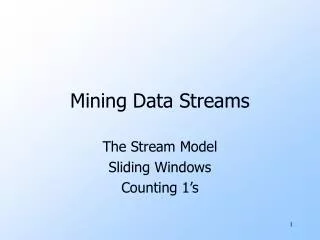
Data Mining for Data Streams Data Mining: Concepts and Techniques
Mining Data Streams • What is stream data? Why Stream Data Systems? • Stream data management systems: Issues and solutions • Stream data cube and multidimensional OLAP analysis • Stream frequent pattern analysis • Stream classification • Stream cluster analysis • Sketching Data Mining: Concepts and Techniques
Characteristics of Data Streams • Data Streams Model: • Data enters at a high speed rate • The system cannot store the entire stream, but only a small fraction • How do you make critical calculations about the stream using a limited amount of memory? • Characteristics • Huge volumes of continuous data, possibly infinite • Fast changing and requires fast, real-time response • Random access is expensive—single scan algorithms(can only have one look) Data Mining: Concepts and Techniques
Continuous Query Architecture: Stream Query Processing SDMS (Stream Data Management System) User/Application Results Multiple streams Stream Query Processor Scratch Space (Main memory and/or Disk) Data Mining: Concepts and Techniques
Stream Data Applications • Telecommunication calling records • Business: credit card transaction flows • Network monitoring and traffic engineering • Financial market: stock exchange • Engineering & industrial processes: power supply & manufacturing • Sensor, monitoring & surveillance: video streams, RFIDs • Web logs and Web page click streams • Massive data sets (even saved but random access is too expensive) Data Mining: Concepts and Techniques
Persistent relations One-time queries Random access “Unbounded” disk store Only current state matters No real-time services Relatively low update rate Data at any granularity Assume precise data Access plan determined by query processor, physical DB design Transient streams Continuous queries Sequential access Bounded main memory Historical data is important Real-time requirements Possibly multi-GB arrival rate Data at fine granularity Data stale/imprecise Unpredictable/variable data arrival and characteristics DBMS versus DSMS Ack. From Motwani’s PODS tutorial slides Data Mining: Concepts and Techniques
Mining Data Streams • What is stream data? Why Stream Data Systems? • Stream data management systems: Issues and solutions • Stream data cube and multidimensional OLAP analysis • Stream frequent pattern analysis • Stream classification • Stream cluster analysis Data Mining: Concepts and Techniques
Processing Stream Queries • Query types • One-time query vs. continuous query (being evaluated continuously as stream continues to arrive) • Predefined query vs. ad-hoc query (issued on-line) • Unbounded memory requirements • For real-time response, main memory algorithm should be used • Memory requirement is unbounded if one will join future tuples • Approximate query answering • With bounded memory, it is not always possible to produce exact answers • High-quality approximate answers are desired • Data reduction and synopsis construction methods • Sketches, random sampling, histograms, wavelets, etc. Data Mining: Concepts and Techniques
Methodologies for Stream Data Processing • Major challenges • Keep track of a large universe, e.g., pairs of IP address, not ages • Methodology • Synopses (trade-off between accuracy and storage) • Use synopsis data structure, much smaller (O(logk N) space) than their base data set (O(N) space) • Compute an approximate answer within a small error range (factor ε of the actual answer) • Major methods • Random sampling • Histograms • Sliding windows • Multi-resolution model • Sketches • Radomized algorithms Data Mining: Concepts and Techniques
Stream Data Processing Methods (1) • Random sampling (but without knowing the total length in advance) • Reservoir sampling: maintain a set of s candidates in the reservoir, which form a true random sample of the element seen so far in the stream. As the data stream flow, every new element has a certain probability (s/N) of replacing an old element in the reservoir. • Sliding windows • Make decisions based only on recent data of sliding window size w • An element arriving at time t expires at time t + w • Histograms • Approximate the frequency distribution of element values in a stream • Partition data into a set of contiguous buckets • Equal-width (equal value range for buckets) vs. V-optimal (minimizing frequency variance within each bucket) • Multi-resolution models • Popular models: balanced binary trees, micro-clusters, and wavelets Data Mining: Concepts and Techniques
Stream Data Mining vs. Stream Querying • Stream mining—A more challenging task in many cases • It shares most of the difficulties with stream querying • But often requires less “precision”, e.g., no join, grouping, sorting • Patterns are hidden and more general than querying • It may require exploratory analysis • Not necessarily continuous queries • Stream data mining tasks • Multi-dimensional on-line analysis of streams • Mining outliers and unusual patterns in stream data • Clustering data streams • Classification of stream data Data Mining: Concepts and Techniques
Mining Data Streams • What is stream data? Why Stream Data Systems? • Stream data management systems: Issues and solutions • Stream data cube and multidimensional OLAP analysis • Stream frequent pattern analysis • Stream classification • Stream cluster analysis • Research issues Data Mining: Concepts and Techniques
Challenges for Mining Dynamics in Data Streams • Most stream data are at pretty low-level or multi-dimensional in nature: needs ML/MD processing • Analysis requirements • Multi-dimensional trends and unusual patterns • Capturing important changes at multi-dimensions/levels • Fast, real-time detection and response • Comparing with data cube: Similarity and differences • Stream (data) cube or stream OLAP: Is this feasible? • Can we implement it efficiently? Data Mining: Concepts and Techniques
Multi-Dimensional Stream Analysis: Examples • Analysis of Web click streams • Raw data at low levels: seconds, web page addresses, user IP addresses, … • Analysts want: changes, trends, unusual patterns, at reasonable levels of details • E.g., Average clicking traffic in North America on sports in the last 15 minutes is 40% higher than that in the last 24 hours.” • Analysis of power consumption streams • Raw data: power consumption flow for every household, every minute • Patterns one may find: average hourly power consumption surges up 30% for manufacturing companies in Chicago in the last 2 hours today than that of the same day a week ago Data Mining: Concepts and Techniques
A Stream Cube Architecture • Atilted time frame • Different time granularities • second, minute, quarter, hour, day, week, … • Critical layers • Minimum interest layer (m-layer) • Observation layer (o-layer) • User: watches at o-layer and occasionally needs to drill-down down to m-layer • Partial materialization of stream cubes • Full materialization: too space and time consuming • No materialization: slow response at query time • Partial materialization… Data Mining: Concepts and Techniques
A Titled Time Model • Natural tilted time frame: • Example: Minimal: quarter, then 4 quarters 1 hour, 24 hours day, … • Logarithmic tilted time frame: • Example: Minimal: 1 minute, then 1, 2, 4, 8, 16, 32, … Data Mining: Concepts and Techniques
Two Critical Layers in the Stream Cube (*, theme, quarter) o-layer (observation) (user-group, URL-group, minute) m-layer (minimal interest) (individual-user, URL, second) (primitive) stream data layer Data Mining: Concepts and Techniques
On-Line Partial Materialization vs. OLAP Processing • On-line materialization • Materialization takes precious space and time • Only incremental materialization (with tilted time frame) • Only materialize “cuboids” of the critical layers? • Online computation may take too much time • Preferred solution: • popular-path approach: Materializing those along the popular drilling paths • H-tree structure: Such cuboids can be computed and stored efficiently using the H-tree structure • Online aggregation vs. query-based computation • Online computing while streaming: aggregating stream cubes • Query-based computation: using computed cuboids Data Mining: Concepts and Techniques
Mining Data Streams • What is stream data? Why Stream Data Systems? • Stream data management systems: Issues and solutions • Stream data cube and multidimensional OLAP analysis • Stream frequent pattern analysis • Stream classification • Stream cluster analysis Data Mining: Concepts and Techniques
Mining Approximate Frequent Patterns • Mining precise freq. patterns in stream data: unrealistic • Even store them in a compressed form, such as FPtree • Approximate answers are often sufficient (e.g., trend/pattern analysis) • Example: a router is interested in all flows: • whose frequency is at least 1% (s) of the entire traffic stream seen so far • and feels that 1/10 of s (ε= 0.1%) error is comfortable • How to mine frequent patterns with good approximation? • Lossy Counting Algorithm (Manku & Motwani, VLDB’02) • Based on Majority Voting… Data Mining: Concepts and Techniques
2 9 9 9 7 6 4 9 9 9 3 9 N = 12; item 9 is majority Majority • A sequence of N items. • You have constant memory. • In one pass, decide if some item is in majority (occurs > N/2 times)? Data Mining: Concepts and Techniques
Misra-Gries Algorithm (‘82) • A counter and an ID. • If new item is same as stored ID, increment counter. • Otherwise, decrement the counter. • If counter 0, store new item with count = 1. • If counter > 0, then its item is the only candidate for majority. Data Mining: Concepts and Techniques
ID ID1 ID2 . . . . IDk count . . A generalization: Frequent Items Find k items, each occurring at least N/(k+1) times. • Algorithm: • Maintain k items, and their counters. • If next item x is one of the k, increment its counter. • Else if a zero counter, put x there with count = 1 • Else (all counters non-zero) decrement all k counters Data Mining: Concepts and Techniques
Frequent Elements: Analysis • A frequent item’s count is decremented if all counters are full: it erases k+1 items. • If x occurs > N/(k+1) times, then it cannot be completely erased. • Similarly, x must get inserted at some point, because there are not enough items to keep it away. Data Mining: Concepts and Techniques
Problem of False Positives • False positives in Misra-Gries algorithm • It identifies all true heavy hitters, but not all reported items are necessarily heavy hitters. • How can we tell if the non-zero counters correspond to true heavy hitters or not? • A second pass is needed to verify. • False positives are problematic if heavy hitters are used for billing or punishment. • What guarantees can we achieve in one pass? Data Mining: Concepts and Techniques
Approximation Guarantees • Find heavy hitters with a guaranteed approximation error [Demaine et al., Manku-Motwani, Estan-Varghese…] • Manku-Motwani (Lossy Counting) • Suppose you want -heavy hitters--- items with freq > N • An approximation parameter , where << .(E.g., = .01 and = .0001; = 1% and = .01% ) • Identify all items with frequency > N • No reported item has frequency < ( - )N • The algorithm uses O(1/ log (N)) memory G. Manku, R. Motwani. Approximate Frequency Counts over Data Streams, VLDB’02 Data Mining: Concepts and Techniques
Window 1 Window 2 Window 3 Lossy Counting Step 1: Divide the stream into ‘windows’ Is window size a function of support s? Will fix later… Data Mining: Concepts and Techniques
Frequency Counts + First Window At window boundary, decrement all counters by 1 Lossy Counting in Action ... Empty Data Mining: Concepts and Techniques
Frequency Counts + Next Window At window boundary, decrement all counters by 1 Lossy Counting continued ... Data Mining: Concepts and Techniques
Error Analysis How much do we undercount? If current size of stream = N andwindow-size = 1/ε then #windows = εN frequency error Rule of thumb: Set ε = 10% of support s Example: Given support frequency s = 1%, set error frequency ε = 0.1% Data Mining: Concepts and Techniques
Output: Elements with counter values exceeding sN – εN Approximation guarantees Frequencies underestimated by at most εN No false negatives False positives have true frequency at least sN – εN How many counters do we need? Worst case: 1/ε log (ε N) counters [See paper for proof] Data Mining: Concepts and Techniques
Enhancements ... Frequency Errors For counter (X, c), true frequency in [c, c+εN] Trick: Remember window-id’s For counter (X, c, w), true frequency in [c, c+w-1] If (w = 1), no error! Batch Processing Decrements after k windows Data Mining: Concepts and Techniques
Stream 28 31 41 34 15 30 23 35 19 Algorithm 2: Sticky Sampling Create counters by sampling Maintain exact counts thereafter What rate should we sample? Data Mining: Concepts and Techniques
Approximation guarantees (probabilistic) Frequencies underestimated by at most εN No false negatives False positives have true frequency at least sN – εN Same error guarantees as Lossy Counting but probabilistic Sticky Sampling contd... For finite stream of length N Sampling rate = 2/Nε log 1/(s) = probability of failure Output: Elements with counter values exceeding sN – εN Same Rule of thumb: Set ε = 10% of support s Example: Given support threshold s = 1%, set error threshold ε = 0.1% set failure probability = 0.01% Data Mining: Concepts and Techniques
Independent of N! Sampling rate? Finite stream of length N Sampling rate: 2/Nε log 1/(s) Infinite stream with unknown N Gradually adjust sampling rate (see paper for details) In either case, Expected number of counters = 2/ log 1/s Data Mining: Concepts and Techniques
No of counters No of counters N (stream length) Sticky Sampling Expected: 2/ log 1/s Lossy Counting Worst Case: 1/ log N Support s = 1% Error ε = 0.1% Log10 of N (stream length) Data Mining: Concepts and Techniques
From elements to setsof elements … Data Mining: Concepts and Techniques
Stream Frequent Itemsets => Association Rules Frequent Itemsets Problem ... • Identify all subsets of items whose current frequency exceeds s = 0.1%. Data Mining: Concepts and Techniques
Three Modules TRIE SUBSET-GEN BUFFER Data Mining: Concepts and Techniques
45 50 40 31 29 32 42 30 50 40 30 31 29 45 32 42 Sets with frequency counts Module 1: TRIE Compact representation of frequent itemsets in lexicographic order. Data Mining: Concepts and Techniques
In Main Memory Module 2: BUFFER Window 1 Window 2 Window 3 Window 4 Window 5 Window 6 Compact representation as sequence of ints Transactions sorted by item-id Bitmap for transaction boundaries Data Mining: Concepts and Techniques
3 3 3 4 2 2 1 2 1 3 1 1 Frequency counts of subsets in lexicographic order Module 3: SUBSET-GEN BUFFER Data Mining: Concepts and Techniques
3 3 3 4 2 2 1 2 1 3 1 1 SUBSET-GEN BUFFER TRIE new TRIE Overall Algorithm ... Problem: Number of subsets is exponential! Data Mining: Concepts and Techniques
SUBSET-GEN Pruning Rules • A-priori Pruning Rule • If set S is infrequent, every superset of S is infrequent. • Lossy Counting Pruning Rule • At each ‘window boundary’ decrement TRIE counters by 1. • Actually, ‘Batch Deletion’: • At each ‘main memory buffer’ boundary, • decrement all TRIE counters by b. See paper for details ... Data Mining: Concepts and Techniques
3 3 3 4 2 2 1 2 1 3 1 1 SUBSET-GEN BUFFER TRIE new TRIE Consumes main memory Consumes CPU time Bottlenecks ... Data Mining: Concepts and Techniques
Design Decisions for Performance TRIE Main memory bottleneck Compact linear array (element, counter, level) in preorder traversal No pointers! Tries are on disk All of main memory devoted to BUFFER Pair of tries old and new (in chunks) mmap() and madvise() SUBSET-GEN CPU bottleneck Very fast implementation See paper for details Data Mining: Concepts and Techniques
Mining Data Streams • What is stream data? Why Stream Data Systems? • Stream data management systems: Issues and solutions • Stream data cube and multidimensional OLAP analysis • Stream frequent pattern analysis • Stream classification • Stream cluster analysis Data Mining: Concepts and Techniques
Classification for Dynamic Data Streams • Decision tree induction for stream data classification • VFDT (Very Fast Decision Tree)/CVFDT (Domingos, Hulten, Spencer, KDD00/KDD01) • Is decision-tree good for modeling fast changing data, e.g., stock market analysis? • Other stream classification methods • Instead of decision-trees, consider other models • Naïve Bayesian • Ensemble (Wang, Fan, Yu, Han. KDD’03) • K-nearest neighbors (Aggarwal, Han, Wang, Yu. KDD’04) • Tilted time framework, incremental updating, dynamic maintenance, and model construction • Comparing of models to find changes Data Mining: Concepts and Techniques
Hoeffding Tree • With high probability, classifies tuples the same • Only uses small sample • Based on Hoeffding Bound principle • Hoeffding Bound (Additive Chernoff Bound) r: random variable R: range of r n: # independent observations Mean of r is at least ravg – ε, with probability 1 – d Data Mining: Concepts and Techniques
Hoeffding Tree Algorithm • Hoeffding Tree Input S: sequence of examples X: attributes G( ): evaluation function d: desired accuracy • Hoeffding Tree Algorithm for each example in S retrieve G(Xa) and G(Xb) //two highest G(Xi) if ( G(Xa) – G(Xb) > ε ) split on Xa recurse to next node break Data Mining: Concepts and Techniques