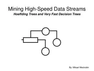
Mining High-Speed Data Streams

Mining High-Speed Data Streams Pedro Domingos Geoff Hulten Sixth ACM SIGKDD International Conference - 2000 Presented by: Tyler J. Sawyer UVM Spring 2014 - CS 332 Data Mining

2 Outline → Introduction → Hoeffding Trees → The VFDT System → Performance Study → Conclusion / Summary → Review Questions

4 Introduction • In today’s society, the ability to extract and interpret knowledge and data quickly and efficiently is an increasingly important task. • Many organizations today have expandable databases that grow at a rate of several million records per day. • Mining these databases yield the following: • Unique opportunities for data analysis • Complex challenges to overcome

5 Introduction - Cont. • Knowledge Discovery Systems are limited by the following: • Time • Memory • Sample Size • Traditional Systems: • Amount of available data is small • Systems use a fraction of their computation power to avoid overfitting • Current Systems: • Bottleneck is time and memory • Majority of sample data is unused; underfitting issues surface.

6 Introduction - Cont. • Today’s Algorithms: • Efficient, but cannot handle supermassive databases. • Current Data Mining systems are not equipped to handle the exponential increase of data expansion • New examples arrive at a higher rate than they can be mined • → Data Corruption!

7 Introduction - Cont. • Requirements for ‘Modern’ Algorithms: • Operate continuously and indefinitely • Incorporate new examples as they become available • Never lose potentially valuable information • Build a model using at most one scan of a database or dataset • Use only a fixed amount of main memory. • Require small, constant time per record. • Make a usable model that can be available at any point during the algorithm’s runtime.

8 Introduction - Cont. • What can fulfill these requirements? • Incremental Learning Methods • Online Methods • Successive Methods • Sequential Methods • While these methods are efficient, they are not always accurate. • These methods rarely recover from a set of unfavorable early examples

10 Hoeffding Trees • Classic Decision Tree Learners • Examples: ID3, C4.5, CART • Assumes examples can be stored simultaneously in main memory; loss of learnable examples. • Disk-based Decision Tree Learners • Examples: SLIQ, SPRINT • Assumes examples are stored on disk. • Big Datasets easily fill disk and errors occur when the dataset is too large to fit.

11 Hoeffding Trees - Cont. • A typical type of Classification Problem • Given : N training examples in the form (x,y) • y = discrete class label • x = vector of d attributes • Goal: Produce a model, y = f(x), to predict classes y of future examples x with high accuracy.

12 Hoeffding Trees - Cont. • Challenge : Design a decision tree learner for extremely large (potentially infinite) datasets with high accuracy and low computational cost. • Given a stream of examples: • The first ones will be used to choose the root test • Succeeding ones will pass to corresponding leaves • Pick the best attributes at each leaf • Continue process recursively

13 Hoeffding Trees - Cont. • But how do we decide how many examples are necessary at each node? • Use a statistical result! • the Hoeffding bound (Chernoff bound)

14 Hoeffding Trees - Cont. • Hoeffding Bound : • G: heuristic measure used to choose test attributes • C4.5 ⇒ information gain • CART ⇒ Gini index • Assume G(.) is to be maximized • G: heuristic measure after seeing n examples • Xa: attribute with the highest observed G • Xb: second-best attribute • △G: difference between Xa and Xb • △G = G(Xa) - G(Xb) > 0 • δ: probability of choosing the wrong attribute

15 Hoeffding Trees - Cont. • The Hoeffding Bound: • after n examples, If △G > ϵ • Xa is the best attribute with probability 1 - δ • Node needs to accumulate examples from the stream until ϵ becomes smaller than △G. • R = range of a real numbered random variables, r • n = independent observations of this variable.

16 Hoeffding Tree Algorithm • Inputs: • S : sequence of examples • X : set of discrete attributes • G(.) : split evaluation function • δ : desired probability of choosing the wrong attribute at any given node • Output: • HT : A decision tree (Hoeffding Tree)

17 Hoeffding Tree Algorithm - Cont.

20 Hoeffding Trees - Cont. • Hoeffding Tree Algorithm guarantees under realistic assumptions the trees generated will be similar to batch learners. • p1 : Leaf Probability (assume this is a constant) • HTδ : Tree produced by HT algorithm with desired δ given an infinite sequence of examples, S. • DT* : Decision tree produced by choosing at each node the attribute with the best G. • △i : Intentional disagreement between two decision trees. • P(x) : Probability that the attribute vector x will be observed. • l(x) : indicator function (1 : True, 0 : False) • ⇒ △i (DT1, DT2) = Σx P(x) l [Path1(x) ≠ Path2(x)] • Theorem 1: E[△i (HTδ,DT*)] < δ / p

21 Hoeffding Trees - Cont. • Suppose Xa and Xb differ by roughly 10%. • According to • δ = 0.1% requires only 380 examples • δ = 0.0001% requires only 345 more examples. • An exponential improvement in δ can be obtained with a linear increase in the number of examples.

23 The VFDT System • Very Fast Decision Tree learner (VFDT) • A decision tree learning system • Based on the Hoeffding Tree algorithm • VFDT allows the use of either information gain or the Gini index as the attribute evaluation measure.

24 The VFDT System - Cont. • Includes a number of refinements to the Hoeffding Tree algorithm: • Ties • G-Computation • Memory • Poor Attributes • Initialization • Rescans

25 The VFDT System - Ties • Two or more attributes may have similar G’s • A large number of examples may be required to decide between them with high confidence. • In this case, the chosen attribute makes little difference. • In a VFDT, we specify a user-threshold, τ • Thus, if △G < ϵ < τ : split on current best attribute.

26 The VFDT System - G-Computation • The most significant part of the time cost per example is recomputing G. • Computing a G value for every new example is inefficient. • In a VFDT, users can specify an nmin value. • nmin : Number of new examples that must accumulate at a leaf before recomputing G.

27 The VFDT System - Memory • a VFDT’s memory use is dominated by the memory required to keep counts for all growing leaves. • If the maximum available memory is reached, VFDT deactivates the least promising leaves. • The least promising leaves are considered to be the ones with the lowest values of plel. • When a leaf is deactivated, its memory is freed, except for a single number used to store the value of plel.

28 The VFDT System - Poor Attributes • a VFDT’s memory usage is also minimized by dropping early on attributes that do not look promising. • As soon as the difference between an attribute’s G and the best one’s becomes greater than ϵ, then the attribute can be dropped. • The memory used to store the corresponding counts can also be freed.

29 The VFDT System - Initialization • VFDT can be initialized with the tree produced by a conventional RAM-based learner on a small subset of the data. • The tree can either be input as it is or over-pruned. • Gives VFDT a “head start”

30 The VFDT System - Rescans • VFDT can rescan previously-seen examples. • Rescans are activated if: • The data arrives slowly enough that time allows for rescans • The dataset is finite and small enough that it is feasible • VFDT will never grow a tree smaller than ones produced by other algorithms.

32 Synthetic Data Study • Comparing VFDT with C4.5 Release 8 • Restricted Two Systems to using the same amount of RAM • VFDT used information gain as the G function. • 14 concepts were used, all with 2 classes and 100 attributes. • For each level after the first 3: • A fraction f of all the nodes were replaced by leaves • The rest became splits on a random attribute. • At depth of 18, all the nodes were replaced with leaves. • Each leaf was randomly assigned a class. • Stream of training examples were then generated • Sampling uniformly from the instance space. • Assigning classes according to the target tree. • Various levels of class and attribute noise was added.

33 Synthetic Data Study - Cont. Accuracy as a function of the number of training examples δ = 10-7 nmin = 200 τ = 5%

34 Synthetic Data Study - Cont. Tree Size as a function of the number of training examples δ = 10-7 nmin = 200 τ = 5%

35 Synthetic Data Study - Cont. Accuracy as a function of the noise level C4.5 : 100k examples, VFDT: 20 million examples

36 Lesion Study Effect of Initializing VFDT with C4.5 with and without pruning

37 Web Data - Trial Run • Application of VFDT to mine the stream of Web Page Requests • Test Location : The Entire University of Washington Campus • δ = 10-7, nmin = 200, τ = 5% • Statistics for mining 1.6 million examples: • VFDT took 1450 seconds to do one pass over the training data • 983 seconds were spent reading data from the disk • C4.5 took 24 hours to mine 1.6 million examples.

38 Web Data - Trial Run Results VFDT Performance on Web Data

40 Conclusion - Hoeffding Trees • A method for learning online • Learns from the increasingly common high-volume data streams • Allows learning in very small constant time per example • Strong guarantees of high asymptotic similarities to corresponding batch trees.

41 Conclusion - VFDT Systems • A high-performance data mining system • Based on Hoeffding trees • Empirical studies show its effectiveness in taking advantage of massive numbers of examples • Practical, efficient, and accurate.

43 Review Questions - 1 of 3 • Question: Name four challenges that modern algorithms have to overcome today. • Answer:See Slide 7. • Operate continuously and indefinitely • Incorporate new examples as they become available • Never lose potentially valuable information • Build a model using at most one scan of a database or dataset • Use only a fixed amount of main memory. • Require small, constant time per record. • Make a usable model that can be available at any point during the algorithm’s runtime.

44 Review Questions - 2 of 3 • Question: List the input requirements of the HT-Algorithm, and state what output is generated. • Answer: See Slide 16 • Inputs: • S : sequence of examples • X : set of discrete attributes • G(.) : split evaluation function • δ : desired probability of choosing the wrong attribute at any given node • Output: • HT : A decision tree (Hoeffding Tree)

45 Review Questions - 3 of 3 • Question: How is memory management handled differently in a VFDT than a Hoeffding Tree? • Answer: See Slide 27 (& 28). • VFDT’s memory use is dominated by the memory required to keep counts for all growing leaves. • If the maximum available memory is reached, VFDT deactivates the least promising leaves. • The least promising leaves are considered to be the ones with the lowest values of plel. • When a leaf is deactivated, its memory is freed, except for a single number used to store the value of plel. • Might also state early-on attributes are dropped for memory efficiency

46 Any Questions? ?

Mining High-Speed Data Streams