Download
1 / 38
380 likes | 531 Vues
Introduction to Biological Modeling. Lecture 3: Metabolism Oct. 6, 2010. Steve Andrews Brent lab, Basic Sciences Division, FHCRC. Last week • modeling cellular dynamics • minimizing necessary parameters • eukaryotic cell cycle • positive feedback, oscillations • databases

E N D
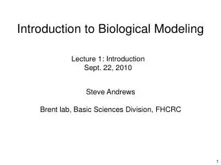
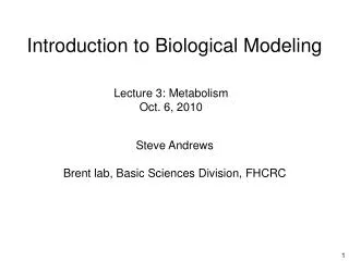
Introduction to Biological Modeling Lecture 3: Metabolism Oct. 6, 2010 Steve Andrews Brent lab, Basic Sciences Division, FHCRC
Last week • modeling cellular dynamics • minimizing necessary parameters • eukaryotic cell cycle • positive feedback, oscillations • databases Copasi software Reading Covert, Schilling, Famili, Edwards, Goryanin, Selkov, and Palsson “Metabolic modeling of microbial strains in silico” TRENDS in Biochemical Sciences 26:179-186, 2001. Klamt, Stelling, “Stoichiometric and constraint-based modeling” in Systems Modeling in Cell Biology edited by Szallasi, Stelling, and Periwal, MIT Press, Cambridge, MA, 2006. Credit: Alberts, et al. Molecular Biology of the Cell, 3rd ed., 1994; http://www.aspencountry.com/product.asp?dept_id=460&pfid=35192.
Small biochemical networks few chemical species few reactions enough known parameters simple dynamics can build model by hand can understand intuitively E. coli chemotaxis eukaryotic cell cycle Credit: Andrews and Arkin, Curr. Biol. 16:R523, 2006; Tyson, Proc. Natl. Acad. Sci. USA 88:7328, 1991.
Big networks (metabolism) Credit: http://www.expasy.ch/cgi-bin/show_thumbnails.pl
Big networks (metabolism) lots of chemical species lots of reactions few known parameters complicated dynamics cannot build model by hand cannot understand intuitively Credit: http://www.expasy.ch/cgi-bin/show_thumbnails.pl
What is and isn’t known A lot is not known • lots of enzymes, reactions, and metabolites • most kinetic parameters • most gene regulation A lot is known • 100s of enzymes • 100s of reactions • 100s of metabolites Databases KEGG Kyoto Encyclopedia of Genes and Genomes BRENDA Braunschweig Enzyme Database unknown reactions reaction sources in a genome-scale H. pylori metabolism model Credit: Covert et al.TRENDS in Biochemical Sciences 26:179, 2001
Why study metabolism? Basic science • how do cells work? • structure of complex networks Medical • metabolic disorders • biosynthetic drugs (e.g. insulin) Bioengineering • biofuels • bioremediation of waste • enzyme production Credits: http://www.autobloggreen.com/2006/05/29/; https://isbibbio.wikispaces.com/Laundry+Detergents+and+Enzymes
Other complex networks biological food webs gene regulatory networks signaling networks non-biological road maps physical internet (IP addresses) internet websites electronic circuits
Metabolism quick overview Anabolism • biosynthesis of proteins, polysaccharides, lipids, etc. Catabolism • breakdown of proteins, polysaccharides, lipids, etc. to make energy credit: http://web.virginia.edu/Heidi/chapter18/chp18.htm
Nomenclature Constraint-based modeling Pathway analysis Metabolic control analysis Copasi Summary
Terminology stoichiometry internal, external metabolites reversible, irreversible reactions enzyme catalysis flux Credit: Klamt and Stelling in System Modeling in Cellular Biology ed. Szallasi et al., p. 73, 2006.
Columns list reaction stoichiometry Example for reaction R10: C + D P + E Stoichiometric matrix Reaction network can be summarized in a matrix reactions Rows list internal metabolite sources and sinks internal metabolites
Dynamical model Dynamics for A reaction rates (fluxes) r1(t) = rate of reaction R1 r2(t) = rate of reaction R2 ... r10(t) = rate of reaction R10
Dynamical model Dynamics for A reaction rates (fluxes) r1(t) = rate of reaction R1 r2(t) = rate of reaction R2 ... r10(t) = rate of reaction R10 math c = metabolite concentrations N = stoichiometric matrix r(t) = reaction rate vector stoichiometric matrix
Nomenclature Constraint-based modeling Pathway analysis Metabolic control analysis Copasi Summary
r2 r2 r1 r1 Constraint-based modeling Main idea We can infer a lot about the fluxes, just from the diagram (and assumptions). • can predict metabolite production rates • can infer missing reactions • improves network understanding before modeling after modeling flux space 1 dimension for each reaction (10 here) everything is possible a few things are possible
Constraint 0: conservation relations Some metabolite concentrations always change together Biology traffic analogy 6 metabolites 5 degrees of freedom total number of cars on island is constant Conservation relations are always true (regardless of dynamics, reaction directionality, etc.)
R5 R6 R7 R8 R9 R10 A B C D E P Constraint 0: conservation relations - math Conservation relations arise when rows of the stoichiometric matrix are linearly dependent Example i.e. there exists yT for which: In this case, the only solution is 6 metabolites 5 degrees of freedom which implies yT is the left null-space of N
Constraint 1: steady-state assumption If system is at steady state, fluxes into and out of each metabolite are equal. biology traffic analogy electronics true when metabolic reactions are much faster than: • external metabolite changes • internal gene regulation current entering and leaving a junction are equal (Kirchoff’s law) the same number of cars enter and leave each intersection.
Constraint 1: steady-state assumption If system is at steady state, fluxes into and out of each metabolite are equal. math R1 R2 R3 R4 R5 R6 R7 R8 R9 R10 biology r is null-space of N Only possible fluxes are proportional to a column of r, or a sum of columns. Uses: • identifies “dead-end” metabolites, which show network mistakes • in computer modeling
Constraint 2: reaction direction, capacity flux signs are known for irreversible reactions flux values may be limited biology traffic analogy irreversible reactions Vmax for enzymes max. transport rates e.g. r1 > 0 traffic is limited by: one-way roads maximum road capacity
math assumes only A is available R1 R2 R3 R4 R5 R6 R7 R8 R9 R10 Constraint 2: reaction direction, capacity flux signs are known for irreversible reactions flux values may be limited biology irreversible reactions Vmax for enzymes max. transport rates
Constraint 3: experimental data Flux measurements can constrain system traffic analogy Measure (bold lines): R1 = R3 = 2, R4 = 1 Infer (dashed lines): R2 = R7 = R9 = R10 = 1 Don’t know (thin lines): R5, R6, or R8
Assume network has evolved to be “optimal” Popular choices: • maximum growth rate per substrate consumed • total flux is minimized (to minimize enzyme synthesis) • for mutants, least change from wild type “Constraint” 4: optimization biology traffic analogy Assume everyone drives the shortest route possible. i.e. total flux is minimized We believe the network evolved to maximize P output. Thus, if it’s just fed A, the fluxes must be as shown (except for R5, R6, R8 uncertainty).
r2 r2 r2 r1 r1 r1 Constraint-based modeling summary Constraints 0. conservation relations steady state assumption max. and min. fluxes experimental data optimization before modeling some constraints more constraints optimized r2 r1 “line of optimality” “flux cone” From the reaction network, and some assumptions, we can estimate most reaction fluxes.
oxygen uptake rate flux cone acetate uptake rate Literature example Edwards, Ibarra, and Palsson, 2001 “In silico predictions of E. coli metabolic capabilities are consistent with experimental data” constraint-based modeling flux cone optimization for maximum growth rate Result • constraint-based modeling and optimization based on growth rate yields fluxes that agree with experiment Credits: Edwards, et al., Nat. Biotechnol. 19:125, 2001.
Nomenclature Constraint-based modeling Pathway analysis Metabolic control analysis Copasi Summary
Pathways Elementary flux mode a path through the network that cannot be simplified (and obeys constraints like steady-state, reaction directionality, etc.)
Pathway applications Removing all essential pathways leads to inviability • helpful for understanding mutants • good for designing drug targets Pathways help build intuition • in all biochemistry texts For further analysis • The minimal set of elementary flux modes are the “eigenvectors” of the network Stelling et al. (2002) showed high correlation between fraction of flux modes available in mutants and viability. No flux modes implied inviable. fraction of wild-type flux modes Credit: Stelling et al. Nature 420:190, 2002.
Nomenclature Constraint-based modeling Pathway analysis Metabolic control analysis Copasi Summary
Metabolic control analysis Metabolic control analysis is sensitivity analysis of the reaction network. Same constraints (steady-state, reaction directionality, etc.) biology traffic analogy we want to make E from A, will doubling enzyme 10 help? what about knocking out enzyme 9? if Mercer Street is widened, will that fix congestion? Or just move it to the next traffic light? Credit: http://www.cityofseattle.net/transportation/ppmp_mercer.htm
Metabolic control analysis Common misconception • There is one rate-limiting step Truth • Lots of reactions affect total production rate - upstream reactions in pathway - downstream reactions due to product inhibition Math Flux control coefficient is effect of enzyme amount on flux: r4 is flux in reaction R4, [E10] is enzyme amount in R10. Flux control coefficients are usually between 0 and 1: R10 has no effect R10 is rate-limiting Typical flux control coefficients are 0 to 0.5, with several enzymes sharing most of the control on any flux.
Metabolic control analysis - substrate conc. What happens if an external metabolite concentration changes? traffic analogy biology we want to make E from A, should we increase [A]? does [P] matter? how will traffic change after a football game ends? Response coefficient: Found by summing control coefficients and “enzyme elasticities” for each enzyme
Nomenclature Constraint-based modeling Pathway analysis Metabolic control analysis Copasi Summary
Metabolic modeling example Pritchard and Kell (2002) investigated flux control in yeast glycoloysis They used Gepasi (predecessor to Copasi). This is a Copasi example file: YeastGlycolysis.cps In Copasi, it’s easy to find: • stoichiometric matrix • constraint 0: mass conservation • steady-state concentrations • elementary flux modes • metabolic control analysis coefficients Credit: Pritchard, Kell, Eur. J. Biochem. 269:3894, 2002.
Nomenclature Constraint-based modeling Pathway analysis Metabolic control analysis Copasi Summary
Summary Big networks Useful databases for metabolism KEGG, BRENDA Stoichiometric matrix math representation of network Constraint-based modeling 0. mass conservation 1. steady-state assumption 2. reaction min. & max. fluxes 3. experimental data 4. optimize Metabolic Control Analysis sensitivity of fluxes to parameters Simulation tools Copasi does many of these tasks
Homework Next week’s class is on gene regulatory networks. Class will be in room B1-072/074 Read Milo, Shen-Orr, Itzkovitz, Kashtan, Chklovskii, and Alon, “Network motifs: Simple building blocks of complex networks” Science 298:824, 2002.