Effective Congestion Management in Manufacturing: Queueing Theory and MEC Examples
This lecture explores congestion management in manufacturing settings through various modeling approaches, including waiting line analysis and simulation. We analyze a case with one operator handling two lines for order taking, focusing on call durations, arrival rates, and associated costs. Using queueing theory, we calculate effective service rates, system utilization, and the costs associated with different machines. The analysis incorporates Little's Law to determine the best operational strategies for reducing idle job costs and improving overall profitability.

Effective Congestion Management in Manufacturing: Queueing Theory and MEC Examples
E N D
Presentation Transcript
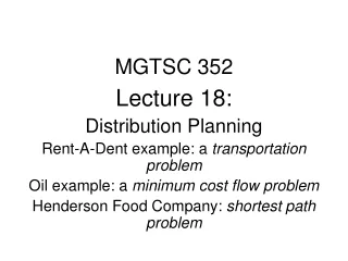
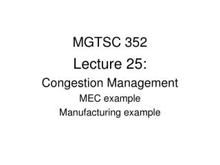
MGTSC 352 Lecture 25: Congestion Management MEC example Manufacturing example
MEC (p. 181) • One operator, two lines to take orders • Average call duration: 4 minutes exp • Average call rate: 10 calls per hour exp • Average profit from call: $24.76 • Third call gets busy signal • How many lines/agents? • Line cost: $4.00/ hr • Agent cost: $12.00/hr • Avg. time on hold < 1 min.
Modeling Approaches • Waiting line analysis template • Simulation • We’ll use both for this example To Excel …
The Laws of Queueing • leff = l (1 – PrBalk) • Effective service rate = entering rate * % sticking around • r = leff /(sm) • utilization = demand / capacity • W = Wq + 1/m • Time in the system = time in the Q + time in service • L = = Lq + S*r • # people in the system = # in the line + # in service • # in service = # servers * probability of server being busy • Little’s Law: L = leffW • Little’s Law for the queue: Lq = leffWq • Little’s Law for the servers: s*r = leff (1/m)
Manufacturing Example (p. 184) Machine (1.2 or 1.8/minute) 1/minute Poisson arrivals Exponential service times
Manufacturing Example • Arrival rate for jobs: 1 per minute • Machine 1: • Processing rate: 1.20/minute • Cost: $1.20/minute • Machine 2: • Processing rate: 1.80/minute • Cost: $2.00/minute • Cost of idle jobs: $2.50/minute • Which machine should be chosen? To Excel …
Manufacturing Example • Cost of machine 1 = $1.20 / min. + ($2.50 / min. / job) (5.00 jobs) = $13.70 / min. • Cost of machine 2 =$2.00 / min. + ($2.50 / min. / job) (1.25 jobs) = $5.13 / min. Switching to machine 2 saves money – reduction in lost revenue outweighs higher operating cost.
Cost of waiting (Mach. 1) • Method 1: • Unit cost × L = ($2.50 / min. job) (5.00 jobs) = $13.70 / min • Method 2: • Unit cost ×× W = = ($2.50 / min. job) (5.00 min) (1 job/min) = $13.70 / min • Little’s LawL = × W
Manufacturing Example 2(p. 184) Changed from 1 to 1.1 Machine (1.2 or 1.8/minute) 1.1/minute Reminder: Cost of idle jobs = holding cost = $2.50 / minute / job Poisson arrivals Exponential service times
Manufacturing Example 3(p. 184) Two machines, each taking twice as long Machine (1.2 or 2 at .6/min) 1/minute Reminder: Cost of idle jobs = holding cost = $2.50 / minute / job Poisson arrivals Exponential service times