Primal Sketch Integrating Structure and Texture
510 likes | 697 Vues
Primal Sketch Integrating Structure and Texture. Ying Nian Wu UCLA Department of Statistics Keck Meeting April 28, 2006. Guo, Zhu, Wu (ICCV, 2003; GMBV, 2004; CVIU, 2006). A Generative Model for Natural Images. texture regions. input image. sketch graph. +. =. synthesized image.

Primal Sketch Integrating Structure and Texture
E N D
Presentation Transcript
Primal Sketch Integrating Structure and Texture Ying Nian Wu UCLA Department of Statistics Keck Meeting April 28, 2006 Guo, Zhu, Wu (ICCV, 2003; GMBV, 2004; CVIU, 2006)
A Generative Model for Natural Images texture regions input image sketch graph + = synthesized image sketchable image synthesized textures
Outline Sparse coding Markov random field Primal sketch model Sketch pursuit algorithm
Sparse Coding Olshausen and Field (1996)
500 bases 800 bases Matching Pursuit Mallat and Zhang (1993) matching pursuit input image
Symbolic representation of 300 bases Reconstructed image Primak sketch
Markov Random Fields Markov Property: MRF model = Gibbs distribution Besag (1974) Geman and Geman (1984) Cross and Jain (1983) One example of neighborhood
MRF model & Image ensemble MRF model (Zhu, Wu & Mumford, 1997) Image ensemble (Wu, Zhu & Liu, 2000)
Feature statistics: histograms of filter responses (Heeger and Bergen, 1995) Filtering – convolution original image I filter responses J of the “dy” filter a set of filters F
800 bases A sample of image ensemble with 5*13=65 parameters 50*70 patch
observed image sampled image from image ensemble Primak sketch
Sparse Coding vs. MRF Sparse Coding models target low complexity patterns. const: related to the dictionary MRF models target high complexity patterns. p*: fitted MRF q: any distribution
Primal Sketch Model Image pixels = Sketchable & Non-sketchable Sketchable: sparse coding using image primitives Non-sketchable: feature statistics/Markov random fields • Integration: • Non-sketchable interpolates sketchable • Non-sketchable recycles failed sketch detections
Sketches Elder and Zucker, 1998
Sketch Graph Sketch graph Vertices: 1,2,3 – corners 4,5,6,7 – end points 8,9,10 – junctions, etc
Image Primitives b) Photometric a) Geometric
Sketch Graph Model Geometric Photometric sketch image
Sketchs = Gabor clusters Alignment across spatial and frequency domains
Integrating structure and texture Sketch Graph Sketches Alignment Gabor filters Non-alignment Textures Pool marginal histograms
Model fitting First: Sketch pursuit aided by Gabors Second: Non-sketchable texturing Sketchability test
Sketch pursuit objective Approximated model
Sketch Pursuit Phase I input image edge/ridge strength Edge/ridge map Proposals: a set of sketches as candidates. Select the sketches in the order of likelihood gain.
Sketch Pursuit Phase IIRefinement Refinement Initialization Evolve the sketch graph by graph operators.
A B Graph Editing A Phase I B Phase II
Phase II Algorithm • Randomly choose a local sub-graph (S0) • Try all 10 pair of graph operators 1~ 5 steps, to generate a set of new graph candidates (S4,S2,S3) • Compare all new graph candidates • Select the one with the largest posterior gain (e.g. S4), accept the new graph. If no positive gain, no update. • Repeat 1~4 until no update S0 G1 G3 S1 S2 S3 G4 S4
texture regions synthesized textures K-mean clustering Histograms in 7x7 window 7 filters x 7 bins
Primal Sketch Model Result input image sketch graph sketchable image reconstructed image
input image sketch graph reconstructed image sketchable image
input image sketch graph reconstructed image
input image reconstructed image sketch graph
Lossy Image Coding codes for the vertices: 152*2*9 = 2,736 bits codes for the strokes: 275*2*4.7 = 2, 585 bits sketch graph codes for the profiles: 275*(2.4*8+1.4*2) = 6,050 bits Total codes for structures (18,185 pixels) 11,371 bits = 1,421 bytes sketchable image
codes for the region boundaries: 3659*3 = 10,977 bits texture regions codes for the texture histograms: 7*5*13*4.5 =2,048 bits Total codes for textures (41,815 pixels) 13,025 bits = 1,628 bytes Total codes for whole image (72,000 pixels), 3,049 bytes synthesized textures
Scaling Wu, Zhu, Bahrami, Li (2006)