POPULATION DYNAMICS
This comprehensive guide covers essential concepts in population dynamics, focusing on data collection and analysis methods. Key topics include measures of central tendency (mean, median, mode, variance, standard deviation), normal distribution, and statistical tests such as Student's t-test and Chi-Square tests. Additionally, it emphasizes the importance of hypothesis testing, outlining procedures for formulating null and alternative hypotheses, the significance level (alpha), and p-values. Gain the foundational knowledge necessary for interpreting data confidently and accurately within the field of population dynamics.


POPULATION DYNAMICS
E N D
Presentation Transcript
POPULATION DYNAMICS Required background knowledge: • Data and variability concepts • Data collection • Measures of central tendency (mean, median, mode, variance, stdev) • Normal distribution and SE • Student’s t-test and 95% confidence intervals • Chi-Square tests • MS Excel
STATISTICS: z-DISTRIBUTION Z = (x – μ) t = (x – μ) σ s x x IF n is very, very large : we use Z distribution to calculate normal deviates If n is not large, we must use t distribution: Equation 3
But first..WHY do we do all this?? Pattern Observation Rigorously Describe Model Explanation or theory (maybe >1) Hypothesis Prediction deduced from model Generate null hypothesis – H0: Falsification test Test • Experiment • IF H0 rejected – model supported • IF H0 accepted – model wrong Integral part of science… HYPOTHESIS TESTING
HYPOTHESIS TESTING α 1.0 0 Not significant p-value Significant These are proportions…if expressed as % You can say with 95% certainty that the pattern you have observed is not due to chance alone You can say with 99% certainty that the pattern you have observed is not due to chance alone • Collect data • Analyse data • Set up hypotheses: • H0 = results are due to CHANCE alone • H1 =results are significant and are not due to chance alone • Test hypotheses: • Determine significance level for hypothesis testing (α) ~ termed ‘Alpha’ • Usually either α = 0.05 or α = 0.01 • Calculate probability value (p) • If p < α then reject H0 ; accept H1 (i.e results are significant and are NOT due to chance alone) • Ifp > α then reject H1; accept H0 (i.e results are not significant and ARE due to chance alone) Measure of certainty 0.05 0.01
POPULATION DYNAMICS Required background knowledge: • Data and variability concepts • Data collection • Measures of central tendency (mean, median, mode, variance, stdev) • Normal distribution and SE • Student’s t-test and 95% confidence intervals • Chi-Square tests • MS Excel
STATISTICS: t-DISTRIBUTION 12 10 8 6 Frequency (%) 4 2 0 0 2 4 6 8 10 12 14 16 18 20 22 24 Height (mm) V = 100 V = 10 V = 5 V = 1 -9 -8 -7 -6 -5 -4 -3 -2 -1 0 1 2 3 4 5 6 7 8 9 t • Because it is based on the normal distribution, the t distribution has all the attributes of the normal distribution: • Completely symmetrical • Area under any part of the curve reflects proportion of t values involved • etc…. Shape of the t distribution varies with v (Degrees of Freedom: n-1): the bigger the n, the less spread the distribution
STATISTICS: t-DISTRIBUTION CONCEPTS α (1) α (1) α (2) 0.1 0.05 0.05 - 2 -4 -3 -1 0 1 2 3 4 -4 -4 -3 -3 - 2 - 2 -1 -1 0 0 1 1 2 2 3 3 4 4 t t t 0.1 H0 : μ = 25 H0 : μ = 25 H1 : μ < 25 H1 : μ≠25 Tails of the t-distribution Example: if our sample size is 11 (v = 10), what is the value of t beyond which 10% (0.1) of the curve is enclosed? – Two possible t-values OR Two-Tailed hypothesis testing One-Tailed hypothesis testing
STATISTICS: T-DISTRIBUTION: CONCEPTS Critical t-value α 1.0 1.0 0 0 Not significant Not significant Measure of certainty 0.05 0.01 Measure of certainty 0.05 p-value 0.01 T-statistic T-statistic compared with critical value Significant Significant α (2) t = (x – μ) - 2 -4 -3 -1 0 1 2 3 4 2.064 -2.064 s x Critical values t Critical values α = 0.05 If t-statistic > 2.064 OR < -2.064 then reject H0 ; accept H1 (i.e results are significant and are NOT due to chance alone)
STATISTICS: T-DISTRIBUTION: CONCEPTS α (1) One-Tailed V=10 α (2) 0.5 0.2 0.1 0.05 0.02 v α (1) 0.25 0.1 0.05 0.025 0.01 0.1 1 1.000 3.078 6.314 12.706 2 0.816 1.886 2.920 4.303 3 0.765 1.638 2.353 3.182 4 0.741 1.533 2.132 2.776 5 0.727 1.476 2.015 2.571 -4 -3 - 2 -1 0 1 2 3 4 6 0.718 1.440 1.943 2.447 -1.372 t 7 0.711 1.415 1.895 2.365 8 0.706 1.397 1.860 2.306 9 0.703 1.383 1.833 1.262 10 0.700 1.372 1.812 2.228 α (2) Two-Tailed 11 0.697 1.363 1.796 2.201 12 0.695 1.356 1.782 2.179 V=10 13 0.694 1.350 1.771 2.160 14 0.692 1.345 1.761 2.145 15 0.691 1.341 1.753 2.131 0.05 16 0.690 1.337 1.746 2.120 0.05 17 0.689 1.333 1.740 2.110 18 0.688 1.330 1.734 2.101 19 0.688 1.328 1.729 2.093 20 0.687 1.325 1.725 2.086 - 2 -4 -3 -1 0 1 2 3 4 21 0.686 1.323 1.721 2.080 22 0.686 1.321 1.717 2.074 t -1.812 1.812 23 0.685 1.319 1.714 2.069 24 0.685 1.318 1.711 2.064 25 0.684 1.316 1.708 2.060 Critical values are found on the t-tables If our sample size is 11 (v = 10), what is the value of t beyond which 10% (0.1) of the curve is enclosed (i.e what is the critical value of t)?
t = (x – μ) t significance level (α 1 or 2), v s x Steps of Student t-tests: • Establish hypotheses (determine if one-tail or two-tailed test • One tail: H0 has > or < in it • Two tail: H0 has ≠ in it • Determine: n, x, μ, s and v (n-1) • Calculate the t-statistic using • Determine significance level for hypothesis testing (α) ~ termed ‘Alpha • Usually either α = 0.05 or α = 0.01 (area in each tail) • Calculate the critical value of t • use T-statistic table, looking up the value for t • Compare t-statistic with critical value to know if you should accept or reject H0
STATISTICS: T-DISTRIBUTION: EXAMPLE Nitrate (after agriculture) x = 24.23 mg.l-1 n= 25 sample tributaries Nitrate (before agriculture) μ = 22 mg.l-1 n= ALL tributaries OBSERVATION MADE: The mean nitrate concentration of water in all the upstream tributaries of a large river prior to intensive agriculture is 22 mg.l-1. Afterwards the mean nitrate concentration in 25 of these tributaries is 24.23 mg.l-1 and s = 4.24 mg.l-1 Based on this observation we want to determine if the intensification of agricultural practices has resulted in a significant change to the nitrate concentration of the freshwater resources. HOW? … Need to determine the probability that a the sample (n = 25, x = 24.23 mg.l-1) could be randomly generated from a population with μ = 22 mg.l-1?
s = √ α (1) α (2) n H0: μ = 22 H0: μ = 22 H1: μ ≠ 22 H1: μ ≠ 22 0.05 0.025 0.025 t = (x – μ) t t = = = 2.629 2.23 (24.23 – 22) One-Tailed Two-Tailed t significance level (α 1 or 2), v 0.848 0.848 4.24 4.24 = = √ 5 25 = 0.848 Go to the hypotheses s s x x Student t-tests: steps for calculation What is the probability that a the sample (n=25, x = 24.23 mg.l-1) could be randomly generated from a population with μ = 22 mg.l-1? • Establish hypotheses • Determine: n, x, μ, s, n and v (n-1) • Calculate the t-statistic • Determine significance level (α) • Calculate the critical value of t • use T-statistic table, looking up the value for t • One tail or two tail? n = 25,x = 24.23, μ = 22.00, s = 4.24,v= 24 t = 2.629 α = 0.05 • Eitherα = 0.05 or α = 0.01 (area in each tail) t 0.05 (α 2), 24
The critical value of t 0.05 (α 2), 24 =2.064 0.025 0.025 -4 -3 - 2 -1 0 1 2 3 4 t -2.064 2.064
STATISTICS: T-DISTRIBUTION: EXAMPLE H0: μ = 22 H1: μ ≠ 22 2.629 0.025 0.025 -4 -3 - 2 -1 0 1 2 3 4 t -2.064 2.064 What is the probability that a the sample (n=25, x = 24.23 mg.l-1) could be randomly generated from a population with μ = 22 mg.l-1? • Establish hypotheses • Determine: n, x, μ, s, n and v (n-1) • Calculate the t-statistic • Determine significance level (α) • Calculate the critical value of t • Compare t-statistic with critical value n = 25,x = 24.23, μ = 22.00, s = 4.24,v= 24 t = 2.629 α = 0.05 Critical value = 2.064 t = 2.629 > critical value SO…means it is very unlikely that a random sample (size 25) would generate a mean of 24.23 mg.l-1 from a population with a mean of 22 mg.l-1 So unlikely, in fact, that we don’t believe it can happen by chance…Reject H0 and accept H1
STATISTICS: T-DISTRIBUTION: EXAMPLES Nitrate (after agriculture) x = 24.23 mg.l-1 n= 25 sample tributaries Nitrate (before agriculture) μ = 22 mg.l-1 n= ALL tributaries What we can then say, is that the before and after nitrate levels in the water are (statistically) significantly different from each other (p < 0.05) We are not making any judgment about whether there is more nitrate in the water after than before, only that the concentrations are different …though some things are self evident!
Q: Is the mean body temperature of this species of crab the same as the ambient air temperature of 24.3 C H0: μ = 24.3 C i.e crab body temp is NOT different from ambient temp H1: μ ≠ 24.3 C i.e crab body temp IS different from ambient temp Now you try… 25 intertidal crabs were exposed to air at 24.3 C, and their body temperatures were measured. • Student-t steps to follow: • Establish hypotheses • Determine: n, x, μ, s, n and v (n-1) • Calculate the t-statistic • Determine significance level (α) • Calculate the critical value of t • Compare t-statistic with critical value
Crab ID Body temp (°C) 1 25.80 2 24.60 3 26.10 4 22.90 5 25.10 6 27.30 7 24.00 8 24.50 9 23.90 10 26.20 11 24.30 12 24.60 13 23.30 14 25.50 15 28.10 16 24.80 17 23.50 18 26.30 19 25.40 Now you try… 20 25.50 21 23.90 22 27.00 23 24.80 24 22.90 Switch to Excel and do the calculations 25 25.40 25 intertidal crabs were exposed to air at 24.3 C, and their body temperatures were measured. Q: Is the mean body temperature of this species of crab the same as the ambient air temperature of 24.3 C • Student-t steps to follow: • Establish hypotheses • Determine: n, x, μ, s, n and v (n-1) • Calculate the t-statistic • Determine significance level (α) • Calculate the critical value of t • Compare t-statistic with critical value
t significance level (α 1 or 2), v Now you try… 25 intertidal crabs were exposed to air at 24.3 C, and their body temperatures were measured. Q: Is the mean body temperature of this species of crab the same as the ambient air temperature of 24.3 C • Student-t steps to follow: • Establish hypotheses • Determine: n, x, μ, s, n and v (n-1) • Calculate the t-statistic • Determine significance level (α) • Calculate the critical value of t • Compare t-statistic with critical value t = 2.7128 α = 0.05
2.173 0.025 0.025 Now you try… -4 -3 - 2 -1 0 1 2 3 4 t -2.064 2.064 > t = 2.7128 Critical value = 2.064 REJECT 25 intertidal crabs were exposed to air at 24.3 C, and their body temperatures were measured. Q: Is the mean body temperature of this species of crab the same as the ambient air temperature of 24.3 C • Student-t steps to follow: • Establish hypotheses • Determine: n, x, μ, s, n and v (n-1) • Calculate the t-statistic • Determine significance level (α) • Calculate the critical value of t • Compare t-statistic with critical value t = 2.713 α = 0.05 Critical value = 2.064 H0: μ = 24.3 C [i.e crab body temp is NOT different from ambient temp] H1: μ ≠ 24.3 C [i.e crab body temp IS different from ambient temp]
POPULATION DYNAMICS Required background knowledge: • Data and variability concepts • Data collection • Measures of central tendency (mean, median, mode, variance, stdev) • Normal distribution and SE • Student’s t-test and 95% confidence intervals • Chi-Square tests • MS Excel
STATISTICS: 95 % CONFIDENCE INTERVALS When we express dispersion around some measure of central tendency, we normally use Standard Deviation: s ± x α (2) In other words, what are limits around our estimate of the population mean, WITHIN which we can be 95% (or 99%) confident that the REAL value of the population mean lies 0.025 0.025 t Two-Tailed To do this, we need a set of t-tables, and V (N-1) s x The t-Distribution allows us to calculate the 95% (or 99%) confidence intervals around an estimate of the population mean
STATISTICS: 95 % CONFIDENCE INTERVALS IF = 42.3 mm n = 26 (V = 25) = 2.15 α (2) 0.025 0.025 * t ά 2 2.06 = 2.15 * - 4.43 mm + 4.43 mm x = 42.3 mm To do this, we need a set of t-tables, and V (n-1) s s s x x x x Then the 95% Confidence Interval (CI) around the mean is calculated as: = 4.429 = 4.429 The Confidence Interval expression is then written as: 42.3 mm ± 4.43 mm i.e we are 95% confident that μ lies between 37.87 and 46.73
POPULATION DYNAMICS Required background knowledge: • Data and variability concepts • Data collection • Measures of central tendency (mean, median, mode, variance, stdev) • Normal distribution and SE • Student’s t-test and 95% confidence intervals • Chi-Square tests • MS Excel
Male Female Blue Red Black White 121.34 g 162.18 g 180.01 g 100 g 200 g 5 people Understanding stats… Types of Data Nominal data – gender, colour, species, genus, class, town, country, model etc Continuous data – concentration, depth, height, weight, temperature, rate etc Discrete data – numbers per unit space, numbers per entity etc The type of data collected influences their statistical analysis
DATA 1 Nominal Continuous Discrete Type + Normal Binomial Poisson…etc 2 Distribution z-tests t-tests ANOVA…etc Choice of statistical test 3 Chi - squared Understanding stats… Data do NOT have to be normally distributed
POPULATION DYNAMICS Required background knowledge: • Data and variability concepts • Data collection • Measures of central tendency (mean, median, mode, variance, stdev) • Normal distribution and SE • Student’s t-test and 95% confidence intervals • Chi-Square tests • MS Excel
16 14 12 You can covert continuous data to discrete data, by assigning data to data classes 10 8 Frequency 6 4 2 0 2 1.2 1.3 1.4 1.5 1.6 1.7 1.8 1.9 2.1 2.2 Height (m) Testing Patterns in Discrete (count) Data: the Chi-Square Test Examples of count data: Number of petals per flower Number of segments per insect leg Number of worms per quadrat Number of white cars on campus…etc
STATISTICS: CHI-SQUARED TESTS [ ] χ χ χ 2 2 2 2 Σ (O – E) = E Equation 4 Hypothesised (EXPECTED) ratio: The bigger the difference between O and E, the greater the ¾ : ¼ 0.75 : 0.25 OR OR When there is no difference will be ZERO = Goodness of Fit n =134 Expected numbers: 100.5 yellow 33.5 green =134 * 0.25 =134 * 0.75 Observed numbers: 113 yellow 21 green OBSERVED ratio: 113 : 21 OR 5.4 : 1 Often want to determine if the population from which you have obtained count data conforms to a certain prediction A geneticist raises a progeny of 134 flowers from this cross: 3 : 1 Where O = Observed, E = Expected Q: Does the OBSERVED ratio differ (SIGNIFICANTLY) from the EXPECTED ratio?
STATISTICS: CHI-SQUARED TESTS [ ] χ 2 2 Σ (O – E) = E Number of categories (K) -1 Steps of X2 tests: • Establish hypotheses • Determine Observed and Expected frequencies • Calculate the X2-statistic using • Determine significance level for hypothesis testing (α = 0.05 or α = 0.01) • Calculate the critical value of X2 • use X2-statistic table • Compare X2-statistic with critical value • If X2-statistic > critical value reject H0 (significant differences between O and E) • If X2-statistic < critical value accept H0 (no significant differences between O and E) Critical value: X2 significance level, v NB: must always usecounts (frequencies) NOT percentages or proportions
STATISTICS: CHI-SQUARED TESTS χ 2 Yellow flowers Green flowers [ ] [ ] (113 – 100.5)2 (21 – 33.5)2 = 1.55 + 4.66 = 6.22 + = 100.5 33.5 Does the OBSERVED ratio (113:21) differ (SIGNIFICANTLY) from the Expected (100.5:33.5) ratio? • Establish hypotheses • H0: Observed and expected ratios are not significantly different • H1: Observed and expected ratios are significantly different • Determine Observed and Expected frequencies • Yellow flowers: Observed = 113 ; Expected = 100.5 • Green flowers: Observed = 21 ; Expected = 33.5 • Calculate the X2-statistic using • Determine significance level for hypothesis testing (α = 0.05 or α = 0.01) • Calculate the critical value of X2 Critical value: X2 significance level, v
Critical value: X2 0.05, 1 Critical value: X2 0.05, v • Degrees of Freedom (v) = K – 1, where K = number of categories • in this case two categories: (yellow-flowering and green-flowering) = (2 – 1) • …therefore v = 1 Critical value = 3.841
STATISTICS: CHI-SQUARED TESTS Q: Does the OBSERVED ratio (113:21) differ (SIGNIFICANTLY) from the Expected (100.5:33.5) ratio? • Establish hypotheses • H0: Observed and expected ratios are not significantly different • H1: Observed and expected ratios are significantly different • Determine Observed and Expected frequencies • Yellow flowers: Observed = 113 ; Expected = 100.5 • Green flowers: Observed = 21 ; Expected = 33.5 • X2-statistic= 6.22 • Determine significance level for hypothesis testing (α = 0.05 or α = 0.01) • Critical value= 3.841 • X2-statistic > critical value therefore reject H0 A: the observed ratio is significantly different from the expected ratio
STATISTICS: CHI-SQUARED TESTS [ ] χ 2 2 Σ (O – E) = E • Establish hypotheses • Determine Observed and Expected frequencies • Calculate the X2-statistic using • Determine significance level for hypothesis testing (α = 0.05 or α = 0.01) • Calculate the critical value of X2 • use X2-statistic table • Compare X2-statistic with critical value • If X2-statistic > critical value reject H0 (significant differences between O and E) • If X2-statistic < critical value accept H0 (no significant differences between O and E) Critical value: X2 significance level, v H0: Population sampled has YS:YW:GS:GW seeds in the ratio 9:3:3:1 H1: Population sampled does not have YS:YW:GS:GW seeds in the ratio 9:3:3:1 Now you try… A plant geneticist has done some crossing between plants and come up with the following numbers of different seeds Q: Has the geneticist sampled from a population having a ratio of 9:3:3:1 ?
STATISTICS: CHI-SQUARED TESTS [ ] χ 2 2 Σ (O – E) = E • Establish hypotheses • Determine Observed and Expected frequencies • Calculate the X2-statistic using • Determine significance level for hypothesis testing (α = 0.05 or α = 0.01) • Calculate the critical value of X2 • use X2-statistic table • Compare X2-statistic with critical value • If X2-statistic > critical value reject H0 (significant differences between O and E) • If X2-statistic < critical value accept H0 (no significant differences between O and E) Critical value: X2 significance level, v Now you try… A plant geneticist has done some crossing between plants and come up with the following numbers of different seeds Q: Has the geneticist sampled from a population having a ratio of 9:3:3:1 ? Switch to Excel
STATISTICS: CHI-SQUARED TESTS χ 2 = 8.97 Now you try… A plant geneticist has done some crossing between plants and come up with the following numbers of different seeds Q: Has the geneticist sampled from a population having a ratio of 9:3:3:1 ? • Establish hypotheses • Determine Observed and Expected frequencies • Calculate the X2-statistic • Determine significance level for hypothesis testing • Calculate the critical value of X2 • use X2-statistic table α = 0.05 Critical value: X2 significance level, v
χ 2 What is the critical value of Critical value: X2 0.05, 3
STATISTICS: CHI-SQUARED TESTS χ 2 = 8.97 Reject the Null Hypothesis that sample drawn from a population showing 9:3:3:1 ratio of YS:YW:GS:GW Now you try… A plant geneticist has done some crossing between plants and come up with the following numbers of different seeds Q: Has the geneticist sampled from a population having a ratio of 9:3:3:1 ? • Establish hypotheses • Determine Observed and Expected frequencies • Calculate the X2-statistic • Determine significance level for hypothesis testing (α = 0.05 or α = 0.01) • Calculate the critical value = 7.815 • Compare X2-statistic with critical value • If X2-statistic > critical value
STATISTICS: CHI-SQUARED TESTS…final word… IF Expected Counts are LESS than ONE, then you must combine the categories NB: By combining data you reduce value of K and also v
POPULATION DYNAMICS Required background knowledge: • Data and variability concepts • Data collection • Measures of central tendency (mean, median, mode, variance, stdev) • Normal distribution and SE • Student’s t-test and 95% confidence intervals • Chi-Square tests • MS Excel
Looking for probabilities: Z-TESTS Comparing two means: T-TESTS Chi - squared Which stats test to use? DATA Discrete Continuous Use Getting started with data.xls for further advice