Download
1 / 50
500 likes | 711 Vues
CS 267: Applications of Parallel Computers Load Balancing. Kathy Yelick www.cs.berkeley.edu/~yelick/cs267_sp07. Outline. Motivation for Load Balancing Recall graph partitioning as load balancing technique Overview of load balancing problems, as determined by Task costs Task dependencies

E N D
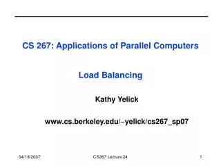
CS 267: Applications of Parallel ComputersLoad Balancing Kathy Yelick www.cs.berkeley.edu/~yelick/cs267_sp07 CS267 Lecture 24
Outline • Motivation for Load Balancing • Recall graph partitioning as load balancing technique • Overview of load balancing problems, as determined by • Task costs • Task dependencies • Locality needs • Spectrum of solutions • Static - all information available before starting • Semi-Static - some info before starting • Dynamic - little or no info before starting • Survey of solutions • How each one works • Theoretical bounds, if any • When to use it CS267 Lecture 24
Load Imbalance in Parallel Applications The primary sources of inefficiency in parallel codes: • Poor single processor performance • Typically in the memory system • Too much parallelism overhead • Thread creation, synchronization, communication • Load imbalance • Different amounts of work across processors • Computation and communication • Different speeds (or available resources) for the processors • Possibly due to load on the machine • How to recognizing load imbalance • Time spent at synchronization is high and is uneven across processors, but not always so simple … CS267 Lecture 24
Measuring Load Imbalance • Challenges: • Can be hard to separate from high synch overhead • Especially subtle if not bulk-synchronous • “Spin locks” can make synchronization look like useful work • Note that imbalance may change over phases • Insufficient parallelism always leads to load imbalance • Tools like TAU can help (acts.nersc.gov) CS267 Lecture 24
Review of Graph Partitioning • Partition G(N,E) so that • N = N1 U … U Np, with each |Ni| ~ |N|/p • As few edges connecting different Ni and Nk as possible • If N = {tasks}, each unit cost, edge e=(i,j) means task i has to communicate with task j, then partitioning means • balancing the load, i.e. each |Ni| ~ |N|/p • minimizing communication volume • Optimal graph partitioning is NP complete, so we use heuristics (see earlier lectures) • Spectral • Kernighan-Lin • Multilevel • Speed of partitioner trades off with quality of partition • Better load balance costs more; may or may not be worth it • Need to know tasks, communication pattern before starting • What if you don’t? CS267 Lecture 24
Load Balancing Overview Load balancing differs with properties of the tasks (chunks of work): • Tasks costs • Do all tasks have equal costs? • If not, when are the costs known? • Before starting, when task created, or only when task ends • Task dependencies • Can all tasks be run in any order (including parallel)? • If not, when are the dependencies known? • Before starting, when task created, or only when task ends • Locality • Is it important for some tasks to be scheduled on the same processor (or nearby) to reduce communication cost? • When is the information about communication known? CS267 Lecture 24
, search Task Cost Spectrum CS267 Lecture 24
Task Dependency Spectrum CS267 Lecture 24
Task Locality Spectrum (Communication) CS267 Lecture 24
Spectrum of Solutions A key question is when certain information about the load balancing problem is known. Leads to a spectrum of solutions: • Static scheduling. All information is available to scheduling algorithm, which runs before any real computation starts. • Off-line algorithms, eg graph partitioning • Semi-static scheduling. Information may be known at program startup, or the beginning of each timestep, or at other well-defined points. Offline algorithms may be used even though the problem is dynamic. • eg Kernighan-Lin • Dynamic scheduling. Information is not known until mid-execution. • On-line algorithms CS267 Lecture 24
Dynamic Load Balancing • Motivation for dynamic load balancing • Search algorithms as driving example • Centralized load balancing • Overview • Special case for schedule independent loop iterations • Distributed load balancing • Overview • Engineering • Theoretical results • Example scheduling problem: mixed parallelism • Demonstrate use of coarse performance models CS267 Lecture 24
Search • Search problems are often: • Computationally expensive • Have very different parallelization strategies than physical simulations. • Require dynamic load balancing • Examples: • Optimal layout of VLSI chips • Robot motion planning • Chess and other games (N-queens) • Speech processing • Constructing phylogeny tree from set of genes CS267 Lecture 24
Example Problem: Tree Search • In Tree Search the tree unfolds dynamically • May be a graph if there are common sub-problems along different paths • Graphs unlike meshes which are precomputed and have no ordering constraints Terminal node (non-goal) Non-terminal node Terminal node (goal) CS267 Lecture 24
Sequential Search Algorithms • Depth-first search (DFS) • Simple backtracking • Search to bottom, backing up to last choice if necessary • Depth-first branch-and-bound • Keep track of best solution so far (“bound”) • Cut off sub-trees that are guaranteed to be worse than bound • Iterative Deepening • Choose a bound on search depth, d and use DFS up to depth d • If no solution is found, increase d and start again • Iterative deepening A* uses a lower bound estimate of cost-to-solution as the bound • Breadth-first search (BFS) • Search across a given level in the tree CS267 Lecture 24
Depth vs Breadth First Search • DFS with Explicit Stack • Put root into Stack • Stack is data structure where items added to and removed from the top only • While Stack not empty • If node on top of Stack satisfies goal of search, return result, else • Mark node on top of Stack as “searched” • If top of Stack has an unsearched child, put child on top of Stack, else remove top of Stack • BFS with Explicit Queue • Put root into Queue • Queue is data structure where items added to end, removed from front • While Queue not empty • If node at front of Queue satisfies goal of search, return result, else • Mark node at front of Queue as “searched” • If node at front of Queue has any unsearched children, put them all at end of Queue • Remove node at front from Queue CS267 Lecture 24
Load balance on 2 processors Load balance on 4 processors Parallel Search • Consider simple backtracking search • Try static load balancing: spawn each new task on an idle processor, until all have a subtree • We can and should do better than this … CS267 Lecture 24
Centralized Scheduling • Keep a queue of task waiting to be done • May be done by manager task • Or a shared data structure protected by locks worker worker Task Queue worker worker worker worker CS267 Lecture 24
Centralized Task Queue: Scheduling Loops • When applied to loops, often called self scheduling: • Tasks may be range of loop indices to compute • Assumes independent iterations • Loop body has unpredictable time (branches) or the problem is not interesting • Originally designed for: • Scheduling loops by compiler (or runtime-system) • Original paper by Tang and Yew, ICPP 1986 • This is: • Dynamic, online scheduling algorithm • Good for a small number of processors (centralized) • Special case of task graph – independent tasks, known at once CS267 Lecture 24
Variations on Self-Scheduling • Typically, don’t want to grab smallest unit of parallel work, e.g., a single iteration • Too much contention at shared queue • Instead, choose a chunk of tasks of size K. • If K is large, access overhead for task queue is small • If K is small, we are likely to have even finish times (load balance) • (at least) Four Variations: • Use a fixed chunk size • Guided self-scheduling • Tapering • Weighted Factoring CS267 Lecture 24
Variation 1: Fixed Chunk Size • Kruskal and Weiss give a technique for computing the optimal chunk size • Requires a lot of information about the problem characteristics • e.g., task costs as well as number • Not very useful in practice. • Task costs must be known at loop startup time • E.g., in compiler, all branches be predicted based on loop indices and used for task cost estimates CS267 Lecture 24
Variation 2: Guided Self-Scheduling • Idea: use larger chunks at the beginning to avoid excessive overhead and smaller chunks near the end to even out the finish times. • The chunk size Ki at the ith access to the task pool is given by ceiling(Ri/p) • where Ri is the total number of tasks remaining and • p is the number of processors • See Polychronopolous, “Guided Self-Scheduling: A Practical Scheduling Scheme for Parallel Supercomputers,” IEEE Transactions on Computers, Dec. 1987. CS267 Lecture 24
Variation 3: Tapering • Idea: the chunk size, Ki is a function of not only the remaining work, but also the task cost variance • variance is estimated using history information • high variance => small chunk size should be used • low variance => larger chunks OK • See S. Lucco, “Adaptive Parallel Programs,” PhD Thesis, UCB, CSD-95-864, 1994. • Gives analysis (based on workload distribution) • Also gives experimental results -- tapering always works at least as well as GSS, although difference is often small CS267 Lecture 24
Variation 4: Weighted Factoring • Idea: similar to self-scheduling, but divide task cost by computational power of requesting node • Useful for heterogeneous systems • Also useful for shared resource clusters, e.g., built using all the machines in a building • as with Tapering, historical information is used to predict future speed • “speed” may depend on the other loads currently on a given processor • See Hummel, Schmit, Uma, and Wein, SPAA ‘96 • includes experimental data and analysis CS267 Lecture 24
When is Self-Scheduling a Good Idea? Useful when: • A batch (or set) of tasks without dependencies • can also be used with dependencies, but most analysis has only been done for task sets without dependencies • The cost of each task is unknown • Locality is not important • Shared memory machine, or at least number of processors is small – centralization is OK CS267 Lecture 24
Distributed Task Queues • The obvious extension of task queue to distributed memory is: • a distributed task queue (or “bag”) • Doesn’t appear as explicit data structure in message-passing • Idle processors can “pull” work, or busy processors “push” work • When are these a good idea? • Distributed memory multiprocessors • Or, shared memory with significant synchronization overhead • Locality is not (very) important • Tasks that are: • known in advance, e.g., a bag of independent ones • dependencies exist, i.e., being computed on the fly • The costs of tasks is not known in advance CS267 Lecture 24
Distributed Dynamic Load Balancing • Dynamic load balancing algorithms go by other names: • Work stealing, work crews, … • Basic idea, when applied to tree search: • Each processor performs search on disjoint part of tree • When finished, get work from a processor that is still busy • Requires asynchronous communication busy idle Service pending messages Select a processor and request work No work found Do fixed amount of work Service pending messages Got work CS267 Lecture 24
How to Select a Donor Processor • Three basic techniques: • Asynchronous round robin • Each processor k, keeps a variable “targetk” • When a processor runs out of work, requests work from targetk • Set targetk = (targetk +1) mod procs • Global round robin • Proc 0 keeps a single variable “target” • When a processor needs work, gets target, requests work from target • Proc 0 sets target = (target + 1) mod procs • Random polling/stealing • When a processor needs work, select a random processor and request work from it • Repeat if no work is found CS267 Lecture 24
How to Split Work • First parameter is number of tasks to split • Related to the self-scheduling variations, but total number of tasks is now unknown • Second question is which one(s) • Send tasks near the bottom of the stack (oldest) • Execute from the top (most recent) • May be able to do better with information about task costs Bottom of stack Top of stack CS267 Lecture 24
Theoretical Results (1) Main result: A simple randomized algorithm is optimal with high probability • Karp and Zhang [88] show this for a tree of unit cost (equal size) tasks • Parent must be done before children • Tree unfolds at runtime • Task number/priorities not known a priori • Children “pushed” to random processors • Show this for independent, equal sized tasks • “Throw balls into random bins”: Q ( log n / log log n ) in largest bin • Throw d times and pick the smallest bin: log log n / log d = Q (1) [Azar] • Extension to parallel throwing [Adler et all 95] • Shows p log p tasks leads to “good” balance CS267 Lecture 24
Theoretical Results (2) Main result: A simple randomized algorithm is optimal with high probability • Blumofe and Leiserson [94] show this for a fixed task tree of variable cost tasks • their algorithm uses task pulling (stealing) instead of pushing, which is good for locality • I.e., when a processor becomes idle, it steals from a random processor • also have (loose) bounds on the total memory required • Chakrabarti et al [94] show this for a dynamic tree of variable cost tasks • works for branch and bound, i.e. tree structure can depend on execution order • uses randomized pushing of tasks instead of pulling, so worse locality • Open problem: does task pulling provably work well for dynamic trees? CS267 Lecture 24
Distributed Task Queue References • Introduction to Parallel Computing by Kumar et al (text) • Multipol library (See C.-P. Wen, UCB PhD, 1996.) • Part of Multipol (www.cs.berkeley.edu/projects/multipol) • Try to push tasks with high ratio of cost to compute/cost to push • Ex: for matmul, ratio = 2n3 cost(flop) / 2n2 cost(send a word) • Goldstein, Rogers, Grunwald, and others (independent work) have all shown • advantages of integrating into the language framework • very lightweight thread creation • CILK (Leiserson et al) (supertech.lcs.mit.edu/cilk) • Space bound on task stealing • X10 from IBM CS267 Lecture 24
Diffusion-Based Load Balancing • In the randomized schemes, the machine is treated as fully-connected. • Diffusion-based load balancing takes topology into account • Locality properties better than prior work • Load balancing somewhat slower than randomized • Cost of tasks must be known at creation time • No dependencies between tasks CS267 Lecture 24
Diffusion-based load balancing • The machine is modeled as a graph • At each step, we compute the weight of task remaining on each processor • This is simply the number if they are unit cost tasks • Each processor compares its weight with its neighbors and performs some averaging • Analysis using Markov chains • See Ghosh et al, SPAA96 for a second order diffusive load balancing algorithm • takes into account amount of work sent last time • avoids some oscillation of first order schemes • Note: locality is still not a major concern, although balancing with neighbors may be better than random CS267 Lecture 24
Mixed Parallelism As another variation, consider a problem with 2 levels of parallelism • course-grained task parallelism • good when many tasks, bad if few • fine-grained data parallelism • good when much parallelism within a task, bad if little Appears in: • Adaptive mesh refinement • Discrete event simulation, e.g., circuit simulation • Database query processing • Sparse matrix direct solvers CS267 Lecture 24
Mixed Parallelism Strategies CS267 Lecture 24
Which Strategy to Use And easier to implement CS267 Lecture 24
Switch Parallelism: A Special Case CS267 Lecture 24
List of CS267 Projects CS267 Lecture 24
CS267 Projects • Matt: Sorting algorithms (UPC impl. & LoPC model) • Nutt & Shoiab: parallel liquid simulation for graphic (PIC and parallel sparse poisson solver) • Jim: Phylogentic tree construction (neighbor joining algorithm); some aspects run in parallel, but large trees don’t fit on single computer (MPI with C) • David, Peter, Steve: Parallel driver for iterative refinement for ScaLAPACK • Jack: Characterizing and scaling material codes for optimal properties (diag large matrices and calc entries) (MPI with Fortran) • JRL: TBD • Narayanan & Statish: Statistical model on GPU (NVIDIA) CS267 Lecture 24
More Projects • Kyle: DNS simulations of lid-driven cavity flow using Chombo (AMR NavStokes Poisson solvers; change current ring vortex changed to lid; “wind on a lake”) (C++ and Fortran with MPI; could you C++ expertise) • Max: Adam’s unstructured multigrid applied to pumice deformation; may modify to take breakage into account. (C with MPI); maybe room for other partners CS267 Lecture 24
Extra Slides CS267 Lecture 24
Simple Performance Model for Data Parallelism CS267 Lecture 24
Modeling Performance • To predict performance, make assumptions about task tree • complete tree with branching factor d>= 2 • d child tasks of parent of size N are all of size N/c, c>1 • work to do task of size N is O(Na), a>= 1 • Example: Sign function based eigenvalue routine • d=2, c=2 (on average), a=3 • Combine these assumptions with model of data parallelism CS267 Lecture 24
Actual Speed of Sign Function Eigensolver • Starred lines are optimal mixed parallelism • Solid lines are data parallelism • Dashed lines are switched parallelism • Intel Paragon, built on ScaLAPACK • Switched parallelism worthwhile! CS267 Lecture 24
Values of Sigma (Problem Size for Half Peak) CS267 Lecture 24
Best-First Search • Rather than searching to the bottom, keep set of current states in the space • Pick the “best” one (by some heuristic) for the next step • Use lower bound l(x) as heuristic • l(x) = g(x) + h(x) • g(x) is the cost of reaching the current state • h(x) is a heuristic for the cost of reaching the goal • Choose h(x) to be a lower bound on actual cost • E.g., h(x) might be sum of number of moves for each piece in game problem to reach a solution (ignoring other pieces) CS267 Lecture 24
Branch and Bound Search Revisited • The load balancing algorithms as described were for full depth-first search • For most real problems, the search is bounded • Current bound (e.g., best solution so far) logically shared • For large-scale machines, may be replicated • All processors need not always agree on bounds • Big savings in practice • Trade-off between • Work spent updating bound • Time wasted search unnecessary part of the space CS267 Lecture 24
Simulated Efficiency of Eigensolver • Starred lines are optimal mixed parallelism • Solid lines are data parallelism • Dashed lines are switched parallelism CS267 Lecture 24
Simulated efficiency of Sparse Cholesky • Starred lines are optimal mixed parallelism • Solid lines are data parallelism • Dashed lines are switched parallelism CS267 Lecture 24