7.1 Polynomial Functions
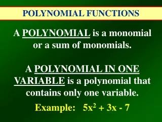
Definition. Recall that a polynomial consists of the sum of one or more monomialsRecall that a monomial is a constant, a variable, or a product of constants and variablesWe say the expression

7.1 Polynomial Functions
E N D
Presentation Transcript
1. 7.1 Polynomial Functions Definition / features
Evaluating for a specific x value
Graphs / end behavior
2. Definition Recall that a polynomial consists of the sum of one or more monomials
Recall that a monomial is a constant, a variable, or a product of constants and variables
We say the expression �3r2 � 3r + 1� is a polynomial in one variable
We generally express polynomials in the form �aoxn + a1xn-1 + a2xn � 2 +�an-1x + an�
In this expression a0, a1, a2, �an represent coefficients
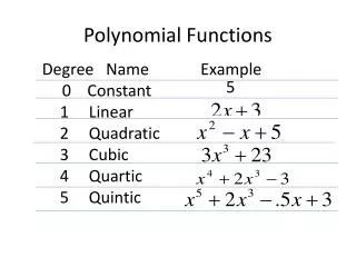
3. Features of the polynomial The DEGREE of a polynomial in one variable is the greatest exponent of its variable
The LEADING COEFFICIENT is the coefficient of the term with the highest degree
For certain degree values, we have names for the corresponding polynomial
4. Types of Polynomials NAME EXAMPLE DEGREE L.C.
Constant 9 0 9
Linear 5x � 2 1 5
Quadratic 3x2 � 4x + 6 2 3
Cubic x3- 8 3 1
Quartic 7x4 + 2x2 � 3x 4 7
Quintic x5 + 111 5 1
5. Example 1-1a
6. Example 1-1b
7. Example 1-1c
8. Example 1-1d
9. Example 1-1e
10. Example 1-1f
11. Example 1-2a
12. Example 1-2d
13. Example 1-3a
14. Example 1-3b
15. Example 1-3c
16. Example 1-3d
17. Example 1-3e
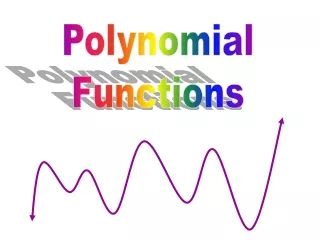
18. Graphs of polynomials Let�s look at some example graphs on the board
We�ll see if we can make some observations about the number of zeroes (a.k.a. x-intercepts), as well as which way the arrows point
19. End behavior Our work with which way the arrows are pointing will help us to describe the end behavior of the function
The end behavior is the behavior of the graph as x approaches positive infinity (i.e., as the graph heads off to the right) and as x approaches negative infinity (i.e., as the graph heads off to the left)
We represent infinity and negative infinity using the symbols 8 and -8
To say �x approaches positive infinity� we write:
x ? 8
20. Analyzing end behavior End behavior is determined by two factors: the degree of the polynomial, and the sign of the lead coefficent
Look at the graphs for polys with degree 1, 3, and 5: do you notice anything about the arrows on the graph?
They point in opposite directions
Look at the graphs for polys with degree 2 and 4: what do you notice?
The arrows point in the same direction (both up or both down)
Whether the arrows both point up or both point down is determined by the sign of the lead coefficient (think in terms of how the sign of �a� affects a parabola)
The LC has a similar effect for odd degree polys
21. FAR-END SUMMARY See the board for a summary of far end behavior
22. Example 1-4a
23. Example 1-4b
24. Example 1-4c
25. Example 1-4d
26. Example 1-4e
27. Example 1-4f
28. HOMEWORK ? ? ? Pg. 350
16 � 44 evens
46 � 48