Appendix D: Linearization
Appendix D: Linearization. Small-Signal Linearization Linearization by Feedback. Material covered in the P RESENT L ECTURE is shown in yellow. I. DYNAMIC MODELING Deriving a dynamic model for mechanical, electrical, electromechanical, fluid- & heat-flow systems

Appendix D: Linearization
E N D
Presentation Transcript
Appendix D: Linearization Small-Signal Linearization Linearization by Feedback
Material covered in the PRESENT LECTURE is shown in yellow I. DYNAMIC MODELING • Deriving a dynamic model for mechanical, electrical, electromechanical, fluid- & heat-flow systems • Linearization the dynamic model if necessary II. DESIGN OF A CONTROLLER: Several design methods exist • Classical control or Root Locus Design: Define the transfer function; Apply root locus, loop shaping,… • Modern control or State-Space Design: Convert ODE to state equation; Apply Pole Placement, Robust control, … • Nonlinear control: Apply Lyapunov’s stability criterion
Introduction • Real models usually exhibit nonideal and nonlinear characteristics • Analysis of a system represented by nonlinear partial differential equations, with time varying coefficients is extremely difficult and requires heavy computations • There is no general analytic method available for solving nonlinear systems
Dealing with Nonlinear Systems In general, we can take one of the following three options: • Replace nonlinear elements with “roughly equivalent linear elements”, which often leads to invalid models; • Develop and solve a nonlinear model, which results in most accurate results, BUT the analysis is too expensive since there is no general analytic methods available for solving. • Linearize ( = find a linear model that approximates well, or at least fairly well, a nonlinear one) in order to make possible more efficient analysis and control design based on linear models.
Why are linear good? To summarize: why are linear models useful? • They are easy to compute, understand and visualize. • They give predictable outputs, in time and over iterations • The analysis of linear theory is complete, developed and efficient • Linear differential equations are easy to solve!
What is a Linear Function? • Linear functions are the first type of functions one learns in mathematics, yet there is not one single definition of linearity… • Different answers apply to different contexts, discipline or purposes.
Possible Answers… A linear function is:… • … a function of the general form y = bx + c • … a function whose derivative is a constant • … a function in which the output is proportional to the input • … a straight line? (careful, this only works in 2D representations) Intuitively, linearity means proportionality of the output with respect to a variable. One variable function are most familiar but functions can be linear in many variables, e.g:
The Real World • Learning about linear behavior is good, but how useful is it? Is the real word linear at all? The answer is no most of the time. • Unfortunately, nonlinear dynamics are not fully understood and the best we can do is simulate the real world with linear or low-order approximations. • To be more precise, linear behavior is simulated locally, at a point or along a small interval in space-time, and then the results are extrapolated about the general domain. • That means that some degree of prediction is possible, but yet, we do not know everything about nonlinearity.
Part A: Small-signal Linearization Approximating the function while considering small disturbances around stable equilibrium points
Applications & Method • Small signal linearization method is the most widely used • It is in general done with the help of Taylor series. • The Taylor expansion of a function f(x) around a point is given by:
Linearization around a point • If we define ,the Taylor expansion becomes: • Note that the functions and all the derivatives are evaluated at the linearization point • If is small (i.e. x is close to ), then we may drop the second and higher-order terms as follows:
Functions of several independent variables • For a function f of a single variable, x: • For a function f of two independent variables, x and y:
Around what point is it proper to linearize? • Intuitively, one would say around zero • But the general answer is around stable equilibrium points
Example 1: Pendulum • The dynamic model is given by: • This equation is nonlinear in the displacement angle θ, because ofthe second term on the left side: f(θ)=(g/l) sin θ • Equilibrium position ? It satisfies: • Therefore, at equilibrium:
Example 1: Pendulum (cont’d) • Linearizing f(θ)about , which is such as with small leads to: • Substituting f in the expression above gives: • Linearizing about a stable equilibrium point requires:
Example 1: Pendulum (cont’d) • Recall the dynamic model: where • At the operating point : where • By subtracting the two equations above:
sinx around x = π/2 • The linear approximation of sin x around x = π/2 is a constant
exp (-x) around 0 • The linear approximation of y = exp(-x) around 0 is y = 1-x • Note that as x goes to infinity, y = exp(-x) converges to 0, while y = 1-x diverges to - infinity
Example 2: Double-pendulum • See class’ notes.
Part B: Linearization by Feedback Subtracting the nonlinear terms out of the equation of motion and adding them to the control.
Pros & Cons Gives a linear model • Provided that the computer implementing the control has enough capability to compute the nonlinear terms fast enough • No matter how large the system variable (θ) becomes.
Example: Pendulum • Consider a pendulum subjected to a torque T. The dynamic model is then: • If we compute the Torque T to be: then the motion is described by: • The resulting linear control will provided the values of u, based on the measurement of θ