
SlideServe
Menu
Préférences
© SlideServe · v2026

Feedback(Exact) Linearization

neville avatar
26 diapositives · 476 Views · Nov 08, 2013

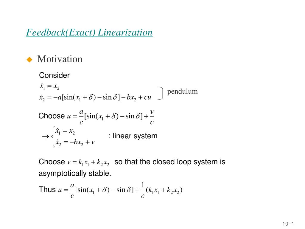
Feedback(Exact) Linearization. Motivation. pendulum. Feedback linearizable system. Advantages The nonlinear control reduces the system to a linear one (exactly). The nonlinear control results in global asymptotically stability of the resulting linear behavior. Disadvantages
Feedback(Exact) Linearization - slide 1
01 / 26Feedback(Exact) Linearization
1 / 17

Télécharger la présentation

Feedback(Exact) Linearization
Une image / un lien ci-dessous est fourni (tel quel) pour télécharger la présentation

Politique de téléchargement : le contenu du site vous est fourni TEL QUEL pour votre information et votre usage personnel ; il ne peut être vendu, concédé sous licence ni partagé sur d’autres sites sans l’accord de son auteur.Le contenu vous est fourni TEL QUEL, pour votre information et votre usage personnel uniquement. Téléchargez la présentation en cliquant sur ce lien. Lors du téléchargement, si vous ne parvenez pas à télécharger une présentation, l’éditeur a peut-être supprimé le fichier de son serveur.Pendant le téléchargement, si vous ne parvenez pas à obtenir une présentation, le fichier a peut-être été supprimé par l’éditeur.

F I N

Plus de contenu associé

Transcription de la présentation
  1. Feedback(Exact) Linearization • Motivation pendulum

  2. Feedback linearizable system • Advantages • The nonlinear control reduces the system to a linear one (exactly). • The nonlinear control results in global asymptotically stability of the resulting linear behavior. • Disadvantages • The real system might be different from the nominal system. Thus the behavior might be nonlinear. • Not every system can be treated this way. • Feedback linearizable system

  3. Feedback linearizable system (Continued) Thus the feedback linearizable systems are of the form : (1) Choose Ex: Is it of the form (1) ? Introduce

  4. Feedback linearizable system (Continued) *

  5. Diffeomorphism Definition: (1) (2)

  6. Calculation of T(·) Also (3)

  7. Calculation of T(·) (Continued) • Two PDEs are the necessary & sufficient conditions for feedback linearization. • T is not unique

  8. Calculation of T(·) (Continued)

  9. Calculation of T(·) (Continued)

  10. Calculation of T(·) (Continued) (i)

  11. Calculation of T(·) (Continued) (ii)

  12. (5) Calculation of T(·) (Continued) (4)

  13. Example Ex:

  14. Example (Continued)

  15. Example (Continued)

  16. Robustness

  17. Stability Analysis

  18. Stability Analysis (Continued) Ex:

  19. Stability Analysis (Continued)

  20. + _ linearization loop pole-placement Closed-loop system  Closed-loop system under feedback(exact) linearization

  21. Input-Output Linearization Let’s consider the tracking problem where and its derivative upto a sufficiently high order are assumed to be known and bounded. Objective : To make tracks while keeping the whole state bounded. An apparent difficulty with this system is that the output is only indirectly related to the input through the state variable and the nonlinear state equation. One might guess that the difficulty of the tracking control design can be reduced if we can find a direct and simple relation between the system output and the control input

  22. Example Ex: Let’s differentiate the output (1) (2) where (2) represents an explicit relationship between and Choose (3) where is a new input to be determined.

  23. Example (Continued) Then Let , then choosing the new input as (where are positive) Then the tracking error of closed loop is (4) which represents an exponentially stable error dynamics. Note : (i) The control law is defined everywhere except that (ii) Full state measurement is necessary in implementing the control law because (3) requires the value of One must remember that (4) only accounts for part of the closed loop dynamics, because it has only order 2, while the whole dynamics has order 3. Thus, a part of the system dynamics has been rendered unobservable in the input-output linearization. We call it internal dynamics.

  24. Example (Continued) For the above example, the internal dynamics is represented by If this internal dynamics is stable (by which we actually mean stability in BIBO), our tracking control problem has indeed been solved. Otherwise, it will end up with burning-up fuses or violent vibration of mechanical members Therefore, the effectiveness of the above control design, based on the reduced order model, hinges upon the stability of the internal dynamics.

  25. Example Ex: Assume that the control objective is to make track Since we know we choose the control law (1) (2) Then The same control input is applied to the second equation leading to the internal dynamics We know that is guaranteed to be bounded by (2) and is assumed to be bounded. Then

  26. Example (Continued) Thus we conclude that since when when Therefore (1) represents a satisfactory tracking control law. If we need to differentiate the output times to generate an explicit relationship between the output and the input , the system is said to have relative degree . If the relative degree of a system is the same as its order, then there is no internal dynamics. In this case, input-output linearization leads to input-state linearization and output tracking can be achieved easily.