Exact Computation
Exact Computation. Theory and Techniques. Serge Adamowsky & Lina Ourima Seminar Algorithmen WS 03 / 04. Contents. Evaluating One Determinant Expression Error-bounds Versus Precision-bounds Error-Bounds Precision-bounds Theory of Exact Computation. Evaluating One Determinant Expression.

Exact Computation
E N D
Presentation Transcript
Exact Computation Theory and Techniques Serge Adamowsky & Lina Ourima Seminar Algorithmen WS 03 / 04
Contents • Evaluating One Determinant Expression • Error-bounds Versus Precision-bounds • Error-Bounds • Precision-bounds • Theory of Exact Computation
Evaluating One Determinant Expression • View Expression as labled dag (=directed acyclic graph) • Each sink node is a number • Each internal node is an operator
Error-bounds Bottom-up Deterministic Depends on error of input Precision-bounds Top down Not deterministic User-specified quantity Error-bounds Versus Precision-bounds
Error Bounds • Number Representation (Notation) • Normalizing Error Digits • Examples for Normalization • Algorithms for Maintaining bigFloat Ranges • Addition • Multiplication • Square Root
Number Representation (Notation) bigFloats used as aproximation b = 1212/343434 0.35 * 10-2 bigFloats used with error-bounds: b‘ = (0.35 0.01) * 10-2 = (35, -2, 1) (f, e, d) := f d*Be The number is exact when d = 0
Normalizing Error Digits • (35, -2, 1)2 = (1225, -4, 71) • Storing many insignificant digits is a waste of space and time Number is normalized when f doesnt start with 0 and 0 d < B Delayed normalization improves accuracy
Algorithms for Maintaining bigFloat Ranges • Addition • Multiplication • Square root With a global precision bound (gpb) c‘ = a‘ b‘: the system produces the most accurate range without the exceeding global p. bound
Addition A safe Algorithm: • Align the least significant bits • Add the digits and error values • Normalize (123, 0, 1) + (246, -2, 3) (12300, 0, 100) + (246, -2, 3) = (12546, 0, 103) Normalized: (125, 0, 2)
Addition Problem: far more digits computed then nessesary Solution: Find the least significant bit (gpb, magnitude of both summands) and don‘t use smaller bits (123, 0, 1) + (2, -2, 1) = (125, 0, 2)
Multiplication (f1, e1, d1) * (f2, e2, d2) = (f1 f2, e1+ e2, f1 d2+ f2 d1+ e1 e2) If f1, f2 positive f1 and f2 (both n digits) not exact => result doesnt have 2n but n significant digits Don‘t compute more digits then the significant ones (like in Addition)
Square Root Newton iteration: i+1½ii 1 ,2,... converges toward i would be exact but Might be not exact and operations can‘t be done accurate still lies between i and i+1
Composite Precision Bounds X approximates x • absolute precision(AP): |X-x| 2-a • relative precision(RP): |X-x| |x| 2-r • composite precision(CP): |X-x| max(2-a, |x| 2-r) written: X = x[a,r] CP AP r = CP RP a =
Algorithms • Most significant bit (MSB) mx :=log|x| • mx[a,r] = MX 2Mx |x| < 21+Mx + max{2e-r, 2a} • Computing Mx is expensive • Often a lower bound for Mx is sufficient
Theory of Exact Computation • Computation of semi-algebraic problems is theoretically possible. • An algebraic number(AN) is any complex root of a polynomial (with integer coefficients) • 2 is AN, since it is root of x2-2 • Isolating interval representation: 2 = (x2-2, [1,2])
Semi-algebraic Predicates (x1, ..., xn) is a Boolean combination of P(x1, ..., x) p 0 p {=, <, >, , } Example: 0(x, y) : (x2 + y2 -1 < 0) (x + y -5 = 0) Is the union of an open disc and a straight line
Tarski Formula A first-order formula based on semi-algebraic predicates is a true Tarski sentence. Example: (x)(y)0(x,y) Sets defined by Tarski formulas are semi-algebraic.
Practical Use? Theorem: A semi-algebraic problem can be solved in double-exponential time on a Turing-machine. • Mainly of theoretical interest • Practical use if some instances can be computed quickly (double exponential time is worst case)
Theory of Root Bounds • Comparing values is a basic operation • It is sufficient to compare to zero determine the sign of an expression • How can we know a number is 0 without looking at infinite signs and without using „some heuristic cut-off epsilon value“?
Detecting Zero • h is a height bound on • The height of an algebraic number is the maximum value of the coefficients in its minimal polynomial • Cauchy‘s bound says: is non-zero iff || > 1 / (1+h) • Evaluate to an AP of 1+log(1+h) to determine the sign