Decision Analysis
Decision Analysis. Under Risk and Uncertainty. Six Steps in Decision-Making. Six Steps: Example. John Thompson Lumber Company. Thompson Lumber (cont.). Types of Decision-Making Environments. Decision-Making Under Uncertainty. Possible criteria comprise. The Maximax Criterion.

Decision Analysis
E N D
Presentation Transcript
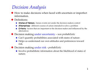
Decision Analysis Under Risk and Uncertainty
Six Steps: Example John Thompson Lumber Company
Decision-Making Under Uncertainty Possible criteria comprise..
The Maximax Criterion Find the maximum (highest) possible outcome for each alternative, then choose the alternative with the maximum (highest) maximum.
The Maximin Criterion Find the minimum (lowest) value in each possible state of nature, and then choose the alternative with the maximum (highest) minimum.
The Criterion of Realism First, select an “alpha” 0 ≤ α ≤ 1, where the closer α is to 1, the more optimistic the decision-maker is. Weighted Average = α(max in row) + (1 – α)(min in row) Realism α = 0.8 Using α = 0.8 124,000 Realism 76,000 0
The Equally Likely Criterion Simply assume that each state of nature is equally likely. Therefore, just get the average value of each alternative and choose the maximum (highest).
The Minimax Regret Criterion For each possible state of nature, determine the best alternative and note its outcome. Then, calculate how much you would regret not having chosen that alternative. (That is your “regret”.) Then, using the “regret table”, find the alternative that minimizes the maximum regret. (See next two slides.)
Decision-Making Under Risk Under conditions of risk, the probability of each state of nature is known. Therefore, by multiplying each possible monetary outcome by its associated probability, an Expected Monetary Value (EMV) can be calculated.
Example (cont.): Calculating EMV with pr(f) = pr(u) = 0.5 Question: Would or could the decision change of the probabilities where different. For example, what if pr(f) = 0.8 and pr(u) = 0.2? EMV 10,000 40,000 0
Expected Value of Perfect Information To get the EVPI, first (a) determine which alternative would be chosen under each state of nature, then (b) calculate the expected value of always making that best alternative choice. In the example, Thompson would choose to construct a large plant if he knew that conditions would be favorable, and no plant if he knew that conditions would be unfavorable. With pr(f) = pr(u) = 0.5, the expected value with perfect information = 0.5x($200,000) + 0.5($0) = $100,000. 10,000 40,000 0
The EVPI (cont.) The expected value of perfect information equals the expected value with perfect information, less the maximum expected market value without perfect information. That is EVPI = EV with perfect info – max EMV From the previous slide and table 3.9. EVPI = $100,000 - $40,000 = $60,000
Minimizing Expected Opportunity Loss (EOL): An alternative to maximizing EMV The EOL is calculated from the “regret matrix” presented above. Each “regret” amount is multiplied by its associated probability and added together to get the EOL. The chosen alternative is the one that minimizes the EOL.
Sensitivity Analysis Rather than choosing the best alternative for given probabilities, one could analyze how EMV changes as a function of the probability (of the good state of nature). Sensitivity analysis can be visualized (as on the next slide) by graphing expected monetary value (EMV) against probability (p). The steeper the EMV line, the more sensitive is EMV to changes in p.
Complex Decision Tree Analysis Decision trees are particularly useful when there are many sequential decisions and/or states of nature in the problem. Consider again Thompson Lumber. But suppose the company has an opportunity to conduct a survey before deciding whether or not to build a manufacturing plant. The survey may either positive or negative results, but in any case will get more accurate payoffs and probabilities. The next slide shows the structure of the tree diagram. The subsequent slide shows the EMVs when the cost of the $10,000 survey is subtracted from the expected profits.
Money and the Utility of Money Suppose you owned a lottery ticket with a 50-50 chance of willing $5, and somebody offered you $2m for it. Would you sell it? Yes or no.
Expected Utility and Utility of Expectation There are two different values, the expected utility of a gamble E[U( )], as described above, and the utility of the expected monetary value of the gamble U(EMV).
Example: Consider a gamble where a person has a 20% chance of winning $1,000 and an 80% chance of winning $200. Also, suppose his/her utility function can be represented by the function U($) = ($)0.5. EMV = (20% x $1,000) + (80% x $200) = $360 U(EMV) = U($360) = ($360)0.5 = 18.97 E[U( )] = (20% x U($1,000)) + (80% x U($200)) = (20% x ($1,000)0.5) + (80% x ($200)0.5)) = (20% x 31.62) + (80% x 14.14) = 17.63 Since U(EMV) > E[U( )], this person prefers the expected value of the gamble to the gamble itself, and is said to be “risk averse”.
Deriving Utility Functions U($) Consider the simple gamble presented below. Choose different values for the certain, Other outcome (Alternative 2) between the best and worst outcomes of Alternative 1, and find the probability of the best outcome “p” at which the person is indifferent between the two alternatives.
Example: Jane Dickson’s Gamble - $10,000 or $0. If the alternative to the gamble had a certain no-risk payout of $5,000, say, Jane wound need a probability of 0.80 of winning $10,000 to be exactly indifferent to the two alternatives.
Example (cont.): Using other possible Alternative 2 certain outcomes, a utility function can be constructed.
Attitudes to Risk – A Graphic Presentation Risk Seeker Risk Avoiders E[U( )] Risk Indifferent U(EMV) E[U( )] > U(EMV) U(EMV) > E[U( )] U(EMV) = E[U( )] E[U( )] U(EMV)
Example: Risk-Seeker Mark Takes a Gamble Clearly, a risk-indifferent or risk-avoiding individual would not take this gamble. But what about Mark?
To answer this, we need to (a) derive Mark’s utility function – shown below – and (b) solve for E[( )] and U(EMV). If don’t play U($0) = 0.15 If play, U( ) = 0.45xU(10,0-00) + 0.55xU(-10,000)