Logistic Population Growth Models
Explore the logistic differential equation model for population growth, considering carrying capacity and environmental limitations. Learn about equilibrium solutions, stability, and separation of variables. Apply the model to analyze deer population growth scenarios.

Logistic Population Growth Models
E N D
Presentation Transcript
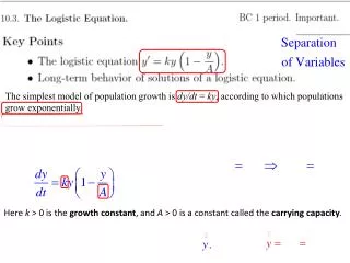
The simplest model of population growth is dy/dt = ky, according to which populations grow exponentially. This may be true over short periods of time, but it is clear that no population can increase without limit. Therefore, population biologists use a variety of other differential equations that take into account environmental limitations to growth such as food scarcity and competition between species. One widely used model is based on the logistic differential equation: Here k > 0 is the growth constant, and A > 0 is a constant called the carrying capacity. Our next slide shows a typical S-shaped solution of a logistic differential equation. As in the previous section, we also denote dy/dt by
Solutions of the logistic equation with y0 < 0 are not relevant to populations because a population cannot be negative (see Exercise 18). Next Slide
The slope field shows clearly that there are three families of solutions, depending on the initial value y0 = y (0). • If y0 > A, then y (t) is decreasing and approaches A as t → ∞. • If 0 < y0 < A, then y (t) is increasing and approaches A as t → ∞. • If y0 < 0, then y (t) is decreasing and Slope field for
has constant solutions: y = 0 and y = A. They correspond to the roots of ky(1 − y/A) = 0, and they satisfy because when y is a constant. Constant solutions are called equilibrium or steady-state solutions. The equilibrium solution y = A is a stable equilibrium because every solution with initial value y0 close to A approaches the equilibrium y = A as t → ∞. By contrast, y = 0 is an unstable equilibrium because every nonequilibrium solution with initial value y0 near y = 0 either increases to A or decreases to −∞. Graph
Having described the solutions qualitatively, let us now find the nonequilibrium solutions explicitly using separation of variables. Assuming that y 0 and yA, we have
For t = 0, we have a useful relation between C and the initial value y0= y (0): As C 0, we may divide by Cekt to obtain the general nonequilibrium solution:
Deer Population A deer population grows logistically with growth constant k = 0.4 year−1 in a forest with a carrying capacity of 1000 deer. (a) Find the deer population P(t) if the initial population is P0 = 100. (b) How long does it take for the deer population to reach 500? `