The solar magnetic cycle
890 likes | 1.05k Vues
Dynamo tutorial Part 1 : solar dynamo models [Paul] Part 2 : Fluctuations and intermittency [Dario] Part 3 : From dynamo to interplanetary magnetic field [Paul].

The solar magnetic cycle
E N D
Presentation Transcript
Dynamo tutorialPart 1 : solar dynamo models [Paul]Part 2 : Fluctuations and intermittency [Dario]Part 3 : From dynamo to interplanetary magnetic field [Paul] ISSI May 2012
Dynamo tutorialPart 1 : solar dynamo modelsThe solar cycle magnetic fieldGlobal 3D MHD simulations 2D axisymmetric solar dynamo models Mean-field electrodynamics and models Babcock-Leighton modelsModels based on HD/MHD instabilities ISSI May 2012
The solar magnetic cycle ISSI May 2012
Maxwell’s equations ISSI May 2012
From Maxwell to MHD (1) Step 1: Drop displacement current to revert to the original form of Ampère’s Law: Step 2: Write down Ohm’s Law in a frame co-moving with the fluid: Step 3: Non-relativistic transformation back to the laboratory frame of reference: ISSI May 2012
From Maxwell to MHD (2) Step 4: Combine with Ampère’s Law to express the electric field as: Step 5: Substitute into Faraday’s Law to get the justly famous magnetohydrodynamical induction equation: where we defined the magnetic diffusivity as: ISSI May 2012
The MHD equations ISSI May 2012
Global 3D MHD simulations ISSI May 2012
Simulation framework Simulate anelastic convection in thick rotating fluid shell, convectively unstable in upper two thirds, using EULAG-MHD in « ideal » mode. This type of ILES simulation is often refered to as « minimally diffusive »; This allows to reach a maximally turbulent state on a given mesh; A flow or magnetic structure can develop gradients reaching the mesh scale and remain nonlinearly stable; Simulations can be run in strongly turbulent regimes over very long times. ISSI May 2012
Kinetic and magnetic energies (120 s.d.=10 yr) ISSI May 2012
Magnetic cycles (1) Large-scale organisation of the magnetic field takes place primarily at and immediately below the base of the convecting fluid layers ISSI May 2012
Zonally-averaged Bphi at r/R =0.718 Magnetic cycles (1) Zonally-averaged Bphi at -58o latitude ISSI May 2012
Successesandproblems KiloGauss-strength large-scale magnetic fields, antisymmetric about equator and undergoing regular polarity reversals on decadal timescales. Cycle period four times too long, and strong fields concentrated at mid-latitudes, rather than low latitudes. Internal magnetic field dominated by toroidal component and strongly concentrated immediately beneath core-envelope interface. Well-defined dipole moment, well-aligned with rotation axis, but oscillating in phase with internal toroidal component. Reasonably solar-like internal differential rotation, and solar-like cyclic torsional oscillations (correct amplitude and phasing). On long timescales, tendency for hemispheric decoupling, and/or transitions to non-axisymmetric oscillatory modes. ISSI May 2012
REALITY CHECKThe numerical treatment of unresolved scales influences a lot the global dynamo behavior ! ISSI May 2012
Axisymmetric+kinematic formulation of solar dynamo models ISSI May 2012
Model setup Solve MHD induction equation in spherical polar coordinates for large-scale (~R), axisymmetric magnetic field in a sphere of electrically conducting fluid: Evolving under the influence of a steady, axisymmetric large-scale flow: Match solutions to potential field in r > R . ISSI May 2012
Kinematic axisymmetric dynamo ISSI May 2012
Differential rotation Slow Fast ISSI May 2012
Shearing by axisymmetricdifferential rotation ISSI May 2012
Kinematic axisymmetric dynamo ISSI May 2012
Meridional circulation ISSI May 2012
REALITY CHECKMany independent global MHD simulations suggest that magnetic backreaction on large-scale flows is an important (perhaps the dominant) amplitude-limiting mechanism ISSI May 2012
Kinematic axisymmetric dynamo ISSI May 2012
Kinematic axisymmetric dynamos ISSI May 2012
Poloidal source terms Turbulent alpha-effect Active region decay (Babcock-Leighton mechanism) Helical hydrodynamical instabilities Magnetohydrodynamical instabilities (flux tubes, Spruit-Tayler) ISSI May 2012
REALITY CHECKWe are forcing fundamentally non-axisymmetric processes into an axisymmetric model formulation ISSI May 2012
Mean-field electrodynamicsand dynamo models ISSI May 2012
The basic idea[ Parker, E.N., ApJ, 122, 293 (1955) ] Cyclonic convective updraft/downdrafts acting on a pre-existing toroidal magnetic field will twist the fieldlines into poloidal planes (in the high Rm regime) The collective effect of many such events is the production of an electrical current flowing parallel to the background toroidal magnetic field; such a current system contributes to the production of a poloidal magnetic component ISSI May 2012
Scale separation Separate flow and magnetic field into large-scale, « laminar » component, and a small-scale, « turbulent » component: Assume now that a good separation of scales exists between these two components, so that it becomes possible to define an averaging operator: such that: This is NOT a linearization!No assumption is made at this stage with regards to the relative magnitudes of flow and field components ISSI May 2012
The turbulent EMF (1) Substitute into MHD induction equation and apply averaging operator: with : TURBULENT ELECTROMOTIVE FORCE ! Now subtract averaged induction equation from original induction equation to obtain evolution equation for b : with : Still no approximation !! ISSI May 2012
The turbulent EMF (2) Now, the whole point of the mean-field approach is NOT to have to deal explicitly with the small scales; since the PDE for b is linear, with the term acting as a source; therefore there must exit a linear relationship between b and B, and also between B and ; We develop the mean emf as Where the various tensorial coefficients can be a function of , of the statistical properties of u, on the magnetic diffusivity, but NOT of . Specifying these closure relationships is the crux of the mean-field approach ISSI May 2012
The alpha-effect (1) Consider the first term in our EMF development: If u is an isotropic random field, there can be no preferred direction in space, and the alpha-tensor must also be isotropic: This leads to: The mean turbulent EMF is parallel to the mean magnetic field! This is called the « alpha-effect » ISSI May 2012
The alpha-effect (2) Computing the alpha-tensor requires a knowledge of the statistical properties of the turbulent flow, more precisely the cross-correlation between velocity components; under the assumption that b << B, if the turbulence is only mildly anisotropic and inhomogeneous, the so-called Second-Order Correlation Approximation leads to where is the correlation time for the turbulence. The alpha-effect is proportional to the fluid helicity! If the mild-anisotropy is provided by rotation, and the inhomogeneity by stratification, then we have ISSI May 2012
Turbulent pumping What if turbulence is significantly anisotropic and/or inhomogeneous? Separate the alpha-tensor into symmetric and antisymmetric parts: where This now leads to: The antisymmetric contributions to the alpha-tensor amount to an advective velocity a, so that the total U in the induction equation becomes . This additional velocity component is known as turbulent pumping ISSI May 2012
Turbulent diffusivity Turn now to the second term in our EMF development: In cases where u is isotropic, we have , and thus: The mathematical form of this expression suggests that can be interpreted as a turbulent diffusivity of the large-scale field. for homogeneous, isotropic turbulence with correlation time , it can be shown that This result is expected to hold also in mildly anisotropic, mildly inhomogeneous turbulence. In general, ISSI May 2012
REALITY CHECKAll commonly-used formulations for the alpha and beta-tensors apply to physical regimes that are far removed from solar interior conditions ISSI May 2012
Scalings and dynamo numbers Length scale: solar/stellar radius: Time scale: turbulent diffusion time: 0 Three dimensionless groupings have materialized: ISSI May 2012
The mean-field zoo The alpha-effect is the source of both poloidal and toroidal magnetic components; works without a large-scale flow! planetary dynamos are believed to be of this kind. Differential rotation shear is the source of the toroidal component; the alpha-effect is the source of only the poloidal component. the solar dynamo is believed to be of this kind. Both the alpha-effect and differential rotation shear contribute to toroidal field production; stellar dynamos could be of this kind if differential rotation is weak, and/or if dynamo action takes place in a very thin layer. ISSI May 2012
Linear alpha-Omega solutions (1) Solve the axisymmetric kinematic mean-field alpha-Omega dynamo equation in a differentially rotating sphere of electrically conducting fluid, embedded in vacuum; in spherical polar coordinates: Choice of alpha: ISSI May 2012
Linear alpha-Omega solutions (2) The growth rate, frequency, and eigenmode morphology are completely determined by the product of the two dynamo numbers ISSI May 2012
Linear alpha-Omega solutions (3) Positive alpha-effect Negative alpha-effect ISSI May 2012
Linear alpha-Omega solutions (4) Time-latitude « butterfly » diagram [ http://solarscience.msfc.nasa.gov/images/bfly.gif ] Equivalent in axisymmetric numerical model: constant-r cut at r/R=0.7, versus latitude (vertical) and time (horizontal) ISSI May 2012
Linear alpha-Omega solutions (5) ISSI May 2012
Stix-Yoshimura sign rule (1) Propagation direction of « dynamo waves » given by: ISSI May 2012
Stix-Yoshimura sign rule (2) Source of B proportional to curl(A) Source of A proportional to B Sinks of A and B proportional to nabla (A,B) ISSI May 2012
Nonlinear models: alpha-quenching (1) We expect that the Lorentz force should oppose the cyclonic motions giving rise to the alpha-effect; We also expect this to become important when the magnetic energy becomes comparable to the kinetic energy of the turbulent fluid motions, i.e.: This motivates the following ad hoc expression for « alpha-quenching »: ISSI May 2012
Nonlinear models: alpha-quenching (2) ISSI May 2012
Nonlinear models: alpha-quenching (3) The magnetic diffusivity is the primary determinant of the cycle period ISSI May 2012
Nonlinear models: alpha-quenching (4) Magnetic fields concentrated at too high latitude; Try instead a latitudinal dependency for alpha: ISSI May 2012
Nonlinear models: alpha-quenching (5) ISSI May 2012