Aggregate Demand and Supply in Economics
420 likes | 431 Vues
Explore the models and factors that explain short-run GDP fluctuations, price levels, and economic growth. Learn about aggregate demand and supply, wealth effects, shifts in demand curve variables, and more.

Aggregate Demand and Supply in Economics
E N D
Presentation Transcript
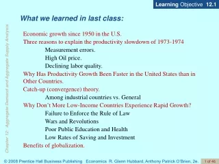
Learning Objective 12.1 What we learned in last class: Economic growth since 1950 in the U.S. Three reasons to explain the productivity slowdown of 1973-1974 Measurement errors. High Oil price. Declining labor quality. Why Has Productivity Growth Been Faster in the United States than in Other Countries. Catch-up (convergence) theory. Among industrial countries vs. General Why Don’t More Low-Income Countries Experience Rapid Growth? Failure to Enforce the Rule of Law Wars and Revolutions Poor Public Education and Health Low Rates of Saving and Investment Benefits of globalization.
Aggregate Demand and Aggregate Supply Learning Objectives To understand why FedEx and other firms are affected by the business cycle, we need to explore the effects that recessions and expansions have on production, employment, and prices.
Learning Objective 12.1 Aggregate Demand Aggregate demand and aggregate supply model A model that explains short-run fluctuations in real GDP and the price level. FIGURE 12.1 Aggregate Demand and Aggregate Supply
Learning Objective 12.1 Aggregate Demand Aggregate demand curve A curve that shows the relationship between the price level and the quantity of real GDP demanded by households, firms, and the government. Short-run aggregate supply curve A curve that shows the relationship in the short run between the price level and the quantity of real GDP supplied by firms.
Learning Objective 12.1 Aggregate Demand Why Is the Aggregate Demand Curve Downward Sloping? GDP has four components: consumption (C), investment (I), government purchases (G), and net exports (NX). If we let Y stand for GDP, we can write the following: AD=Y = C + I + G + NX The Wealth Effect: How a Change in the Price Level Affects Consumption The impact of the price level on consumption is called the wealth effect.
Learning Objective 12.1 Aggregate Demand Why Is the Aggregate Demand Curve Downward Sloping? The Interest-Rate Effect: How a Change in the Price Level Affects Investment The impact of the price level on investment is known as the interest-rate effect. The International-Trade Effect: How a Change in the Price Level Affects Net Exports The impact of the price level on net exports is known as the international-trade effect.
Learning Objective 12.1 Aggregate Demand Shifts of the Aggregate Demand Curve versusMovements Along It An important point to remember is that the aggregate demand curve tells us the relationship between the price level and the quantity of real GDP demanded, holding everything else constant.
Learning Objective 12.1 Aggregate Demand The Variables That Shift the Aggregate Demand Curve The variables that cause the aggregate demand curve to shift fall into three categories: • Changes in government policies • Changes in the expectations of households and firms • Changes in foreign variables Don’t Let This Happen to YOU!Be Clear Why the Aggregate Demand Curve Is Downward Sloping
Learning Objective 12.1 Aggregate Demand The Variables That Shift the Aggregate Demand Curve Changes in Government Policies Monetary policy The actions the Federal Reserve takes to manage the money supply and interest rates to pursue macroeconomic policy objectives. Fiscal policy Changes in federal taxes and purchases that are intended to achieve macroeconomic policy objectives, such as high employment, price stability, and high rates of economic growth.
Learning Objective 12.1 Aggregate Demand The Variables That Shift the Aggregate Demand Curve Changes in the Expectations of Households and Firms If households become more optimistic about their future incomes, they are likely to increase their current consumption. Changes in Foreign Variables If firms and households in other countries buy fewer U.S. goods or if firms and households in the United States buy more foreign goods, net exports will fall, and the aggregate demand curve will shift to the left.
Learning Objective 12.1 MakingtheConnection In a Global Economy, How Can You Tell the Imports from the Domestic Goods? Is the Toyota Sienna as American as apple pie?
Learning Objective 12.1 12-1 Solved Problem Movements along the Aggregate Demand Curve versus Shifts of the Aggregate Demand Curve
Learning Objective 12.1 Aggregate Demand The Variables That Shift the Aggregate Demand Curve Changes in Foreign Variables Table 12-1 Variables That Shift the Aggregate Demand Curve
Learning Objective 12.1 Aggregate Demand The Variables That Shift the Aggregate Demand Curve Changes in Foreign Variables Table 12-1 Variables That Shift the Aggregate Demand Curve (continued)
Learning Objective 12.2 Aggregate Supply The Long-Run Aggregate Supply Curve Long-run aggregate supply curve A curve that shows the relationship in the long run between the price level and the quantity of real GDP supplied. LRAS=Potential real GDP or Full employment GDP. Changes in the price level do not affect potential real GDP. Three factors affecting potential real GDP: Technological change Labor force Capital stock
Learning Objective 12.2 Aggregate Supply The Long-Run Aggregate Supply Curve FIGURE 12.2 The Long-Run Aggregate Supply Curve
Learning Objective 12.2 Aggregate Supply The Short-Run Aggregate Supply Curve The three most common explanations as to why a short-run aggregate supply curve slopes upward include: 1 Contracts make some wages and prices “sticky.” 2 Firms are often slow to adjust wages. 3 Menu costs make some prices sticky. Menu costs The costs to firms of changing prices.
Learning Objective 12.2 Aggregate Supply Shifts of the Short-Run Aggregate Supply Curve versus Movements Along It It is important to remember the difference between a shift in a curve and a movement along a curve. Variables That Shift the Short-Run Aggregate Supply Curve Increases in the Labor Force and in the Capital Stock Technological Change Expected Changes in the Future Price Level
Learning Objective 12.2 Aggregate Supply Variables That Shift the Short-Run Aggregate Supply Curve Expected Changes in the Future Price Level FIGURE 12.3 How Expectations of the Future Price Level Affect the Short-Run Aggregate Supply
Learning Objective 12.2 Aggregate Supply Variables That Shift the Short-Run Aggregate Supply Curve Adjustments of Workers and Firms to Errors in Past Expectations about the Price Level Unexpected Changes in the Price of an Important Natural Resource Supply shock An unexpected event that causes the short-run aggregate supply curve to shift.
Learning Objective 12.2 Aggregate Supply Variables That Shift the Short-Run Aggregate Supply Curve Unexpected Changes in the Price of an Important Natural Resource Table 12-2 Variables That Shift the Short-Run Aggregate Supply Curve
Learning Objective 12.2 Aggregate Supply Variables That Shift the Short-Run Aggregate Supply Curve Unexpected Changes in the Price of an Important Natural Resource Table 12-2 Variables That Shift the Short-Run Aggregate Supply Curve (continued)
Learning Objective 12.3 What we learned in last class: Curves!! We learned only two things: AD, LRAS and SRAS: Definitions and slopes Variables that shift those curves !!
Learning Objective 12.3 Macroeconomic EquilibriumIn the Short Run Using AD and SRAS curves to analyze how changes in economic conditions and policies affect real GDP and the price level (in short-run). Examples: Fed lowered interest rate. Bush lifts oil drill ban. Obama proposes to lower income tax on working-family. Bush’s tax-rebate program. I.T. innovation. Immigrants flow to the U.S. Declining labor quality ……, ……
Learning Objective 12.3 Macroeconomic Equilibriumin the Long Run and the Short Run FIGURE 12.4 Long-Run Macroeconomic Equilibrium
Learning Objective 12.3 Macroeconomic Equilibriumin the Long Run and the Short Run Recessions, Expansions, and Supply Shocks Because the full analysis of the aggregate demand and aggregate supply model can be complicated, we begin with a simplified case, using two assumptions: 1 The economy has not been experiencing any inflation. The price level is currently 100, and workers and firms expect it to remain at 100 in the future. 2 The economy is not experiencing any long-run growth. Potential real GDP is $10.0 trillion and will remain at that level in the future.
Learning Objective 12.3 Macroeconomic Equilibriumin the Long Run and the Short Run Recessions, Expansions, and Supply Shocks Recession FIGURE 12.5 The Short-Run and Long-Run Effects of a Decrease in Aggregate Demand
Learning Objective 12.3 Macroeconomic Equilibriumin the Long Run and the Short Run Recessions, Expansions, and Supply Shocks Expansion FIGURE 12.6 The Short-Run and Long- run Effects of an Increase in Aggregate Demand
Learning Objective 12.3 Macroeconomic Equilibriumin the Long Run and the Short Run Recessions, Expansions, and Supply Shocks Supply Shock Stagflation A combination of inflation and recession, usually resulting from a supply shock.
Learning Objective 12.3 Macroeconomic Equilibriumin the Long Run and the Short Run Recessions, Expansions, and Supply Shocks Supply Shock FIGURE 12.7 The Short-Run and Long-Run Effects of a Supply Shock
Learning Objective 12.4 A Dynamic Aggregate Demandand Aggregate Supply Model We can create a dynamic aggregate demand and aggregate supply model by making three changes to the basic model. • Potential real GDP increases continually, shifting the long-run aggregate supply curve to the right. • During most years, the aggregate demand curve will be shifting to the right. • Except during periods when workers and firms expect high rates of inflation, the short-run aggregate supply curve will be shifting to the right.
Learning Objective 12.4 A Dynamic Aggregate Demandand Aggregate Supply Model FIGURE 12.8 A Dynamic Aggregate Demand and Aggregate Supply Model
Learning Objective 12.4 A Dynamic Aggregate Demandand Aggregate Supply Model What Is the Usual Cause of Inflation? FIGURE 12.9 Using Dynamic Aggregate Demand and Aggregate Supply to Understand Inflation
Learning Objective 12.4 A Dynamic Aggregate Demandand Aggregate Supply Model The Slow Recovery from the Recession of 2001 The recession of 2001 was caused by a decline in aggregate demand. Several factors contributed to this decline: • The end of the stock market “bubble.” • Excessive investment in information technology. • The terrorist attacks of September 11, 2001. • The corporate accounting scandals.
Learning Objective 12.4 MakingtheConnection Does Rising Productivity Growth Reduce Employment?
Learning Objective 12.4 A Dynamic Aggregate Demandand Aggregate Supply Model The Economy in 2007: Continuing Expansion or Looming Recession? In late 2007, economists were divided over whether the twin blows of higher oil prices and a declining housing sector would be sufficient to push the economy into a recession. The majority of economists forecast that growth in real GDP would slow but that the economy would not tip into recession.
Learning Objective 12.4 MakingtheConnection Do Oil Shocks Still Cause Recessions? FedEx’s trucks and jets have become more fuel efficient.
Learning Objective 12.4 12-4 Solved Problem Showing the Oil Shock of 1974–1975 on a Dynamic Aggregate Demand and Aggregate Supply Graph
Appendix Keynesian revolution The name given to the widespread acceptance during the 1930s and 1940s of John Maynard Keynes’s macroeconomic model. Macroeconomic Schools of Thought These alternative schools of thought use models that differ significantly from the standard aggregate demand and aggregate supply model. We can briefly consider each of the three major alternative models: 1 The monetarist model 2 The new classical model 3 The real business cycle model
Appendix TheMonetaristModel Macroeconomic Schools of Thought The monetarist model—also known as the neo-Quantity Theory of Money model—was developed beginning in the 1940s by Milton Friedman, an economist at the University of Chicago who was awarded the Nobel Prize in Economics in 1976. Monetary growth rule A plan for increasing the quantity of money at a fixed rate that does not respond to changes in economic conditions. Monetarism The macroeconomic theories of Milton Friedman and his followers; particularly the idea that the quantity of money should be increased at a constant rate.
Appendix The New Classical Model Macroeconomic Schools of Thought The new classical model was developed in the mid-1970s by a group of economists including Nobel laureate Robert Lucas of the University of Chicago, Thomas Sargent of New York University, and Robert Barro of Harvard University. New classical macroeconomics The macroeconomic theories of Robert Lucas and others, particularly the idea that workers and firms have rational expectations.
Appendix The Real Business Cycle Model Macroeconomic Schools of Thought Beginning in the 1980s, some economists, including Nobel laureates Finn Kydland of Carnegie Mellon University and Edward Prescott of Arizona State University, argued that Lucas was correct in assuming that workers and firms formed their expectations rationally and that wages and prices adjust quickly to supply and demand but wrong about the source of fluctuations in real GDP. Real business cycle model A macroeconomic model that focuses on real, rather than monetary, causes of the business cycle.